Currencies

Highlights An inevitable and imminent U.K. general election will be one of the most unpredictable and ‘non-linear’ elections ever. This non-linearity makes it difficult to take a high-conviction view on sterling’s direction because a tiny vote swing in one direction or another could be the difference between a no-deal Brexit – and the pound below parity against the euro – or a solid coalition for remain – and the pound at €1.30. Instead, a good strategy is to buy sterling volatility on the announcement of the election. The easiest way to implement this is simultaneously to buy at-the-money call and put options (versus either the euro or dollar). In a soft Brexit or remain, the U.K. equity sectors most likely to outperform the overall market are real estate and general retailers. In a hard Brexit, a U.K. sector likely to outperform the overall market is clothing and accessories. Feature Chart of the WeekSterling Volatility Could Go Up A Lot
Sterling Volatility Could Go Up A Lot
Sterling Volatility Could Go Up A Lot
Lyndon B Johnson famously said that that the first rule of politics is to learn to count. A government is a lame duck if it does not have a majority of legislators to drive and set its policy. Fifty years on, LBJ’s namesake is learning this first rule of politics. Boris Johnson is running a minority U.K. government. The irony is that this makes it impossible for a pro-Brexit Johnson to pass legislation for the Brexit process itself! Ending the free movement of EU citizens was supposedly one of the biggest ambitions of the Brexit vote. But astonishingly, even after a no-deal Brexit, free movement would not end – because EU law continues to apply until its legal foundation is repealed. The U.K. government wanted to end free movement through a new law, the immigration bill, but the proposed legislation, along with several other key new laws, cannot make it through parliament. The Most Non-Linear Election Looms The only way out of the impasse is to change the parliamentary arithmetic via a snap general election. The trouble is that the outcome of such an election is near impossible to predict. This is because the U.K.’s first past the post electoral system is designed for a head-to-head between two dominant parties. But right now, there are four parties in play – from left to right: Labour, Liberal Democrat, Conservative, and Brexit. While in Scotland, the SNP is resurgent. Making the next U.K. general election one of the most unpredictable and ‘non-linear’ elections ever. The outcome of a snap general election is near impossible to predict. For example, in the recent Brecon and Radnorshire by-election, the 10 percent of votes that went to the Brexit party syphoned just enough ‘leave’ votes from the Conservatives to hand the seat to the Lib Dems. Repeated nationwide, such a swing could inflict mortal damage to the Conservatives. On the other hand, the staunchly pro-remain Lib Dems could also syphon crucial votes from a Labour party that is prevaricating on its Brexit policy. Understanding this, Johnson isn’t using the next election to resolve Brexit; quite the opposite, he is using Brexit to resolve the next election – in his favour – with the ancient strategy of ‘divide and rule’. Unite ‘leave’ by tacking to the hard right, and divide ‘remain’ between Labour, Lib Dem, Green, SNP, and Plaid Cymru. However, it is a very risky strategy. A small but critical rump of Brexit party voters are diehard anti-establishment rather than pure leave votes; furthermore, remainers almost certainly will vote tactically as they did in 2017 when they obliterated the Conservatives’ overall majority. For U.K. investments, the inevitable imminent election dominates all other considerations, as its outcome will determine the U.K.’s ultimate trading relationship with the EU and rest of the world, as well as establish the U.K’s overarching economic policy and strategy. But to reiterate, the outcome is highly non-linear. A tiny vote swing in one direction or another could be the difference between a no-deal Brexit – and the pound below parity against the euro – or a solid coalition for remain – and the pound at €1.30, as sterling’s ‘Brexit discount’ is unwound (Chart I-2 and Chart I-3). Chart I-2Sterling's Brexit Discount Is 15 Percent, Based On Real Interest Rate Differentials...
Sterling's Brexit Discount Is 15 Percent, Based On Real Interest Rate Differentials...
Sterling's Brexit Discount Is 15 Percent, Based On Real Interest Rate Differentials...
Chart I-3...And Expected Interest Rate ##br##Differentials
...And Expected Interest Rate Differentials
...And Expected Interest Rate Differentials
The non-linearity makes it difficult to take a high-conviction view on sterling’s direction. Instead, as soon as an election is announced, a good strategy is to buy sterling volatility. Although it has risen recently, sterling volatility is only in the foothills relative to the heights of 2016, meaning plenty of upside (Chart I-1). The easiest way to implement this is simultaneously to buy at-the-money call and put options (versus either the euro or dollar). Brexit Investments A common question we get is what are the most Brexit-impacted investments, in both directions? As mentioned, the most obvious is sterling. Relative to the established relationship with interest rate differentials prior to the Brexit vote in 2016, the pound now carries a Brexit discount of around 15 percent. For U.K. investments, the inevitable imminent election dominates all other considerations. Related to this, the FTSE100 has outperformed the Eurostoxx600. This is exactly as theory would suggest. The FTSE100 and Eurostoxx600 are just a collection of global multi-currency earning companies quoted in pounds and euros respectively. So when sterling weakens, the multi-currency earnings increase more in FTSE100 index terms than in Eurostoxx600 index terms, resulting in FTSE100 outperformance (Chart I-4). Chart I-4The FTSE100 Outperforms When Sterling Weakens
The FTSE100 Outperforms When Sterling Weakens
The FTSE100 Outperforms When Sterling Weakens
Turning to U.K. equity sectors, those most likely to outperform the overall market in a soft Brexit are real estate and general retailers (Chart I-5 and Chart I-6). Chart I-5U.K. Real Estate Outperforms In A Soft Brexit
U.K. Real Estate Outperforms In A Soft Brexit
U.K. Real Estate Outperforms In A Soft Brexit
Chart I-6U.K. General Retailers Outperform In A Soft Brexit
U.K. General Retailers Outperform In A Soft Brexit
U.K. General Retailers Outperform In A Soft Brexit
While a sector likely to outperform the overall market in a hard Brexit is clothing and accessories (Chart I-7). Chart I-7U.K. Clothing And Accessories Could Outperform In A Hard Brexit
U.K. Clothing And Accessories Could Outperform In A Hard Brexit
U.K. Clothing And Accessories Could Outperform In A Hard Brexit
Four Disruptors Revisited The final section this week revisits the wider context for Brexit and other recent examples of populism. Specifically, they are backlashes to four structural disruptors to economies and financial markets. Disruptor 1: Protectionism. Since the Great Recession, an extremely polarised distribution of economic growth has left many people’s standard of living stagnant – despite seemingly decent headline economic growth and job creation (Chart I-8). Chart I-8Disruptor 1: Income Inequality Leads To Protectionism
Disruptor 1: Income Inequality Leads To Protectionism
Disruptor 1: Income Inequality Leads To Protectionism
Looking to find a scapegoat, economic nationalism and protectionism have resonated very strongly with voters in several major economies: the U.S., U.K., Italy, and Brazil. Other voters could follow in the same vein. But history teaches us that protectionism ends up hurting many more people than it helps. Disruptor 2: Technology. The bigger danger is that the malaise is being misdiagnosed. Many middle-income job losses are not due to globalization, but due to technology. A polarised distribution of economic growth has left many people’s standard of living stagnant. Specifically, Artificial Intelligence (AI) is replacing secure middle-income jobs and displacing workers into insecure low-income manual jobs – like bartending and waitressing – which AI cannot (yet) replace (Table I-1). And AI’s impact on middle-income jobs is only in its infancy.1 The worry is that by misdiagnosing the illness as globalization and wrongly responding with protectionism, the illness will get worse, rather than improve. Table I-1Disruptor 2: Technology
Brexit: Rock Meets Hard Place
Brexit: Rock Meets Hard Place
Disruptor 3: Debt super-cycles have reached exhaustion. Protectionism carries a further danger. Just like developed economies did a decade ago, major emerging market economies are now coming to the end of structural credit booms and need to wean themselves off their credit addictions (Chart I-9). At this point of vulnerability, aggressive protectionism risks tipping these emerging economies into a sharp slowdown. Chart I-9Disruptor 3: Debt Super-Cycles Have Reached Exhaustion
Disruptor 3: Debt Super-Cycles Have Reached Exhaustion
Disruptor 3: Debt Super-Cycles Have Reached Exhaustion
Disruptor 4: Financial markets are richly valued. Disruptors one, two and three come at a time when equities are valued to generate feeble total nominal returns over the next decade (Chart I-10). Extremely compressed risk premiums are justified so long as bond yields remain ultra-low. Otherwise, the rich valuations will come under pressure. Chart I-10Disruptor 4: Financial Markets Are Richly Valued
Disruptor 4: Financial Markets Are Richly Valued
Disruptor 4: Financial Markets Are Richly Valued
The long-term investment message is crystal clear. With the four disruptors in play, we strongly advise long-term investors not to follow passive (equity) index-tracking strategies. Instead, we advise long-term investors to follow bespoke structural investment themes as shown in our structural recommendations section. Please note that owing to my travelling there is no fractal trading system this week. Normal service will resume next week. Dhaval Joshi, Chief European Investment Strategist dhaval@bcaresearch.com Footnotes 1 Please see the European Investment Strategy Special Report ‘The Superstar Economy: Part 2’ January 19, 2017 available at eis.bcaresearch.com Cyclical Recommendations Structural Recommendations Closed Fractal Trades Trades Closed Trades Asset Performance Currency & Bond Equity Sector Country Equity Indicators Bond Yields Chart II-1Indicators To Watch - Bond Yields
Indicators To Watch - Bond Yields
Indicators To Watch - Bond Yields
Chart II-2Indicators To Watch - Bond Yields
Indicators To Watch - Bond Yields
Indicators To Watch - Bond Yields
Chart II-3Indicators To Watch - Bond Yields
Indicators To Watch - Bond Yields
Indicators To Watch - Bond Yields
Chart II-4Indicators To Watch - Bond Yields
Indicators To Watch - Bond Yields
Indicators To Watch - Bond Yields
Interest Rate Chart II-5Indicators To Watch - Interest Rate Expectations
Indicators To Watch - Interest Rate Expectations
Indicators To Watch - Interest Rate Expectations
Chart II-6Indicators To Watch - Interest Rate Expectations
Indicators To Watch - Interest Rate Expectations
Indicators To Watch - Interest Rate Expectations
Chart II-7Indicators To Watch - Interest Rate Expectations
Indicators To Watch - Interest Rate Expectations
Indicators To Watch - Interest Rate Expectations
Chart II-8Indicators To Watch - Interest Rate Expectations
Indicators To Watch - Interest Rate Expectations
Indicators To Watch - Interest Rate Expectations
Feature In investment, there are times when your view and your strategy should not be the same. Our view remains that the global economy is likely to avoid recession over the next 18 months, that the Fed will cut rates once or twice more as an “insurance” but not enter a full easing cycle, that global bond yields will rise, and that risk assets will outperform over the next 12 months. But the risks to that view have increased, and so we want to bolster the hedge against our view being wrong. We don’t see Recommended Allocation
Monthly Portfolio Update: Dialing Down Risk
Monthly Portfolio Update: Dialing Down Risk
Chart 1GAA Portfolio Volatility Relative To Benchmark
GAA Portfolio Volatility Relative To Benchmark
GAA Portfolio Volatility Relative To Benchmark
government bonds as an attractive hedge at this level of yield, and so are moving to a “barbell” strategy, with overweights in equities and cash, and an underweight in fixed income. This lowers the volatility of our recommended portfolio to close to that of the benchmark (Chart 1). First, the good news. Although the manufacturing sector globally continues to deteriorate, with many PMIs falling to below 50, services and consumption remain robust almost everywhere (Chart 2). With central banks easing monetary policy, and in some countries (Italy, the U.S., the U.K., maybe even Germany) governments loosening fiscal policy, financial conditions are improving, which will eventually support growth (Chart 3). Intra-cyclical manufacturing downturns typically last around 18 months, and this one is close to its sell-by date (Chart 4). Chart 2Manufacturing Weak, Services Fine
Manufacturing Weak, Services Fine
Manufacturing Weak, Services Fine
So what has changed? First, manufacturing has continued to decline for longer than we expected. In the early summer, there were signs of a bottoming in Europe, but these are no longer evident. The diffusion index of the global manufacturing PMI (i.e. the percentage of countries with a rising versus falling PMI), which typically leads the PMI by six months, suggests the PMI has further to fall (Chart 5). Chart 3Easing Financial Conditions Will Help
Easing Financial Conditions Will Help
Easing Financial Conditions Will Help
Chart 4Close To The Bottom?
Close To The Bottom?
Close To The Bottom?
Chart 5Further Downside For PMIs?
Further Downside For PMIs?
Further Downside For PMIs?
Chart 6China's Reluctant Monetary Stimulus
China's Reluctant Monetary Stimulus
China's Reluctant Monetary Stimulus
The most likely cause of this is that China has been more reluctant to ramp up monetary stimulus than we expected. It has eased fiscal policy, but monetary policy has been tentative: despite a moderate increase in credit creation this year, M3 money supply growth has barely accelerated (Chart 6). This has been enough to stabilize Chinese growth, but has been insufficient to give the sort of boost to global growth that China provided in 2016. There are two reasons for China’s reluctance to stimulate. The authorities seemingly continue to prioritize debt deleveraging and clamping down on shadow banking. And, also, maybe they do not want to give a boost to the global economy that would help the U.S. avoid recession and increase the probability of President Trump’s being reelected. China has been more reluctant to ramp up monetary stimulus than we expected. The Trade War is an increasing risk. BCA’s geopolitical strategists continue to assign a 40% probability to a resolution by year-end,1 but it is becoming harder to see how (or, indeed, why) President Xi would offer concessions to the U.S. that would lead to a deal. Ultimately, if Chinese growth slows significantly and U.S. stocks fall sharply, China will boost monetary stimulus and President Trump will push for even a superficial trade agreement. But things will need to get worse first. Meanwhile, the rise in global political uncertainty – and the mercurial nature of Trump’s foreign and trade policies – are a risk for markets (Chart 7). Chart 7Global Political Risks Rising
Global Political Risks Rising
Global Political Risks Rising
Chart 8Consumers (Mostly) Remain Confident
Consumers (Mostly) Remain Confident
Consumers (Mostly) Remain Confident
We are also concerned about how long consumption can remain robust in this environment. So far, consumer confidence has remained resilient in the U.S., though it has dipped a little in Europe and Japan (Chart 8). But, if corporate profits remain weak, companies will start to delay hiring decisions and begin to lay off workers. This would be the transmission mechanism for the manufacturing slowdown to spread into the broader economy. So far, fortunately, there are few signs it is happening: German unemployment is at a record low, and U.S. initial claims continue to run at or below last year’s level (Chart 9). Chart 9No Signs Of Weakening Labor Market
No Signs Of Weakening Labor Market
No Signs Of Weakening Labor Market
Table 1GAA Recession Checklist
Monthly Portfolio Update: Dialing Down Risk
Monthly Portfolio Update: Dialing Down Risk
In the recession checklist we have published for the past two or more years, we are starting to have to tick off more warning signs (Table 1 and Chart 10). Chart 10Some Worrying Signs
Some Worrying Signs
Some Worrying Signs
Chart 11Risk Of Recession No Longer Negligible
Risk Of Recession No Longer Negligible
Risk Of Recession No Longer Negligible
For example, the yield curve has inverted both for the 3-month/10 year and 2-year/10-year. Although the yield curve has been an almost infallible predictor of recession in the past 70 years, there are some reasons to argue that it may not be as good this time: for example, central bank purchases have artificially pulled down long-term rates. But inversion is probably a self-fulfilling prophesy. For example, in a recent Fed Senior Bank Loan Officers Survey, 40% of banks said they would tighten credit standards simply because of a moderate inversion of the yield curve. Formal models of recession 12 months ahead that incorporate the yield curve slope, put recession risk now at about 25% (Chart 11). Chart 1218 Months Of Ups And Downs
18 Months Of Ups And Downs
18 Months Of Ups And Downs
Given all this, we think it is appropriate to take some risk off. As far back as February 2018, we argued that “investors primarily concerned with capital preservation might look to dial down risk or hedge exposure now”.2 Given the ups and down of markets in the past 18 months, we suspect that those risk-averse investors would not have been unhappy with that advice (Chart 12), although they would also have missed some nice equity rallies over that time, if they had been nimble enough to time entry and exit points. Since a majority of the subscribers to this service are rather conservative, we are now extending that advice to all clients. On a 12-month time horizon, we raise cash to overweight. We are also reducing somewhat both our equity overweight and bond underweight. In this period of increased uncertainty, a portfolio closer than usual to benchmark makes sense. (BCA’s House View is a little more bullish, remaining neutral on cash and overweight equities on the 12-month horizon). Fixed Income: Absent recession, we see little room for rates to fall further. The U.S. 10-year Treasury yield (now 1.5%) should stay above its July 2016 historic low of 1.37%. The Fed is unlikely to cut rates by 100 basis points over the next 12 months, as futures imply. We would expect only two 25 bp rate cuts: in September and either October or December. Yields are likely eventually to move up over the next 12 months (particularly given that inflation continues to trend higher). But they may not move much for a while, and so we move from underweight to neutral on duration for now. Eventually, we see investors understanding that government bonds are no longer an attractive hedge at current yields. Even if German 10-year yields fell to -1.2% (probably around the lowest possible), one-year total return would only be 5% (Table 2). The U.S. looks a little better, though. One could imagine the yield falling to zero in the next recession, which would give a return of 16%. On credit, we remain neutral: it represents a low-beta play on equities. So far this year, both investment-grade and high-yield bonds have eked out a small positive excess return (Chart 13). Table 2Not Much Room For Positive Returns
Monthly Portfolio Update: Dialing Down Risk
Monthly Portfolio Update: Dialing Down Risk
Chart 13Credit Returns Have Not Been Bad
Credit Returns Have Not Been Bad
Credit Returns Have Not Been Bad
Chart 14Downside For Cyclicals?
Downside For Cyclicals?
Downside For Cyclicals?
Equities: To offset our overweight on equities, we continue with a low-beta country/regional tilt. We recommend an overweight on the U.S., and underweight on Emerging Markets. The key for upside to U.S. equities remains earnings. Analysts have a pessimistic forecast of only 2.5% EPS growth in 2019 for the S&P500. A rough proxy for earnings growth (nominal GDP growth of 4.5%, wage growth of 3.5% leading to some margin expansion, 2% buybacks) points to EPS growth of around 7-8%. Q3 earnings (where analysts forecast -2% year-on-year) are likely to surprise on the upside, as did Q1 and Q2, though the strong dollar and weak overseas growth are risks. In our next Quarterly, to be published on October 1, we may make some adjustments to further dial down risk, for example in our equity sector recommendations, which currently have a slight cyclical tilt. The relative performance of cyclicals has started to wobble, and the message from bond markets is that cyclicals have further to fall in relative terms (Chart 14). Investors will come to understand that government bonds are no longer an attractive hedge at current yields. Currencies: The trade-weighted dollar has broadly moved sideways in the past year (Chart 15), weakening against the yen, but strengthening against the euro and EM currencies. We remain neutral on the dollar. It will continue to be pulled by two opposing forces: weak global growth is a positive, but the Fed has more room to cut rates than the rest of the world and so interest rate differentials will shift against the dollar. The renminbi is likely to continue to weaken, as the Chinese use currency policy as the least painful offset against U.S. tariffs. The latest set of tariffs suggests that the CNY needs to fall to around 7.5-7.6 to the USD to offset their impact but, if Trump implements all the tariffs he has threatened, it could fall as far as 8.0 (Chart 16). This would pull other EM currencies down further. GBP will continue to be buffeted by Brexit scenarios. A no-deal Brexit could bring it down to 1.00 against the USD, whereas Remain or a very soft Brexit would take it back to PPP, 1.43. The current level is a probability weighted average of the two. Chart 15Dollar Has Moved Broadly Sideways
Dollar Has Moved Broadly Sideways
Dollar Has Moved Broadly Sideways
Chart 16CNY Could Fall Much Further
CNY Could Fall Much Further
CNY Could Fall Much Further
Commodities: The oil price has been hurt by a slowing of demand in developed economies (Chart 17). Supply, however, remains tight, and our energy strategists have cut their forecast for Brent this year only modestly to an average of $66 a barrel (from an earlier forecast of $70, and from a current spot price of $60).3 Industrial commodities continue to struggle because of China’s slowdown (Chart 18) and are unlikely to recover until China’s stimulus is beefed up. Gold remains a good insurance for investors worried about geopolitical risk, recession, and inflation. Chart 17EM Oil Demand Has Been Weak
EM Oil Demand Has Been Weak
EM Oil Demand Has Been Weak
Chart 18Industrial Commodities Hurt By China
Industrial Commodities Hurt By China
Industrial Commodities Hurt By China
Garry Evans, Senior Vice President Chief Global Asset Allocation Strategist garry@bcaresearch.com 1 Please see Geopolitical Strategy Weekly, “Big Trouble In Greater China,” dated August 23, 2019, available at gps.bcareseach.com 2 Please see Global Asset Allocation, “GAA Monthly Portfolio Update,” dated February 1, 2018, available at gaa.bcaresearch.com. 3 Please see Commodity & Energy Strategy, “USD Strength Slows Oil Demand Growth; 2020 Brent Forecast Remains At $75/bbl,” dated August 22, 2019, available at ces.bcaresearch.com Recommended Asset Allocation
Highlights While a self-fulfilling crisis of confidence that plunges the global economy into recession cannot be excluded, it is far from our base case. Provided the trade war does not spiral out of control, it is highly likely that global equities will outperform bonds over the next 12 months. The auto sector has been the main driver of the global manufacturing slowdown. As automobile output begins to recover later this year, so too will global manufacturing. Go long auto stocks. As a countercyclical currency, the U.S. dollar will weaken once global growth picks up. We expect to upgrade EM and European equities later this year along with cyclical equity sectors such as industrials, energy, and materials. Financials should also benefit from steeper yield curves. We still like gold as a long-term investment. However, the combination of higher bond yields and diminished trade tensions could cause bullion to sell off in the near term. As such, we are closing our tactical long gold trade for a gain of 20.5%. Feature “The Democrats are trying to 'will' the Economy to be bad for purposes of the 2020 Election. Very Selfish!” – @realDonaldTrump, 19 August 2019 8:26 am “The Fake News Media is doing everything they can to crash the economy because they think that will be bad for me and my re-election” – @realDonaldTrump, 15 August 2019 9:52 am Bad Juju Chart 1Spike In Google Searches For The Word Recession
A Psychological Recession?
A Psychological Recession?
President Trump’s remarks, made just a few days after the U.S. yield curve inverted, were no doubt meant to deflect attention away from the trade war, while providing cover for any economic weakness that might occur on his watch. But does the larger point still stand? Google searches for the word “recession” have spiked recently, even though underlying U.S. growth has remained robust (Chart 1). Could rising angst induce an actual recession? Theoretically, the answer is yes. A sudden drop in confidence can generate a self-fulfilling cycle where rising pessimism leads to less private-sector spending, higher unemployment, lower corporate profits, weaker stock prices, and ultimately, even deeper pessimism. Two things make such a vicious cycle more probable in the current environment. First, the value of risk assets is quite high in relation to GDP in many economies (Chart 2). This means that any pullback in equity prices or jump in credit spreads will have an outsized impact on financial conditions. Chart 2The Total Market Value Of Risk Assets Is Elevated
The Total Market Value Of Risk Assets Is Elevated
The Total Market Value Of Risk Assets Is Elevated
Chart 3Not Much Scope To Cut Rates
Not Much Scope To Cut Rates
Not Much Scope To Cut Rates
Second, policymakers are currently more constrained in their ability to react to adverse shocks, such as an intensification of the trade war, than in the past. Interest rates in Europe and Japan are already at zero or in negative territory (Chart 3). Even in the U.S., the zero-lower bound constraint – though squishier than once believed – remains a formidable obstacle. Chart 4 shows that the Federal Reserve has cut rates by over five percentage points, on average, during past recessions. It would be impossible to cut rates by that much this time around if the U.S. economy were to experience a major downturn. Chart 4The Fed Is Worried About The Zero Bound
The Fed Is Worried About The Zero Bound
The Fed Is Worried About The Zero Bound
Fiscal stimulus could help buttress growth. However, both political and economic considerations are likely to limit the policy response. While China is stimulating its economy, concerns about excessively high debt levels have caused the authorities to adopt a reactive, tentative approach. Japan is set to raise the consumption tax on October 1st. Although a variety of offsetting measures will mitigate the impact on the Japanese economy, the net effect will still be a tightening of fiscal policy. Germany has mused over launching its own Green New Deal, but so far there has been a lot more talk than action. President Trump floated the idea of cutting payroll taxes, only to abandon it once it became clear that the Democrats were unwilling to go along. On The Positive Side Despite these clear risks, we are inclined to maintain our fairly sanguine 12-to-18 month global macro view. There are a number of reasons for this: First, the weakness in global manufacturing over the past 18 months has not infected the much larger service sector (Chart 5). Even in Germany, with its large manufacturing base, the service sector PMI remains above 50, and is actually higher than it was late last year. This suggests that the latest global slowdown is more akin to the 2015-16 episode than the 2007-08 or 2000-01 downturns. Chart 5AThe Service Sector Has Softened Much Less Than Manufacturing (I)
The Service Sector Has Softened Much Less Than Manufacturing (I)
The Service Sector Has Softened Much Less Than Manufacturing (I)
Chart 5BThe Service Sector Has Softened Much Less Than Manufacturing (II)
The Service Sector Has Softened Much Less Than Manufacturing (II)
The Service Sector Has Softened Much Less Than Manufacturing (II)
Second, manufacturing activity should benefit from a turn in the inventory cycle over the remainder of the year. A slower pace of inventory accumulation shaved 90 basis points off of U.S. growth in the second quarter and is set to knock another 40 basis points from growth in the third quarter, according to the Atlanta Fed GDPNow model. Excluding inventories, U.S. GDP growth would have been 3% in Q2 and is tracking at 2.7% in Q3 – a fairly healthy pace given the weak global backdrop (Chart 6). Chart 6The U.S. Economy Is Still Holding Up Well
A Psychological Recession?
A Psychological Recession?
Outside the U.S., inventories are making a negative contribution to growth (Chart 7). In addition to the official data, this can be seen in the commentary accompanying the Markit manufacturing surveys, which suggest that many firms are liquidating inventories (Box 1). Falling inventory levels imply that sales are outstripping production, a state of affairs that cannot persist indefinitely. Third, and related to the point above, the automobile sector has been the key driver of the global manufacturing slowdown. This is in contrast to 2015-16, when the main culprit was declining energy capex. According to Wards, global vehicle production is down about 10% from year-ago levels, by far the biggest drop since the Great Recession (Chart 8). The drop in automobile production helps explain why the German economy has taken it on the chin recently. Chart 7Inventories Are Making A Negative Contribution To Growth
Inventories Are Making A Negative Contribution To Growth
Inventories Are Making A Negative Contribution To Growth
Chart 8Auto Sector: The Culprit Behind The Manufacturing Slowdown
Auto Sector: The Culprit Behind The Manufacturing Slowdown
Auto Sector: The Culprit Behind The Manufacturing Slowdown
Importantly, motor vehicle production growth has fallen more than sales growth, implying that inventory levels are coming down. Despite secular shifts in automobile ownership preferences, there is still plenty of upside to automobile usage. Per capita automobile ownership in China is only one-fifth of what it is in the United States, and one-fourth of what it is in Japan (Chart 9). This suggests that the recent drop in Chinese auto sales will be reversed. As automobile output begins to recover later this year, so too will global manufacturing. Investors should consider going long automobile makers. Chart 10 shows that the All-Country World MSCI automobiles index is trading near its lows on both a forward P/E and price-to-book basis, and sports a juicy dividend yield of nearly 4%.1 Chart 9The Automobile Ownership Rate Is Still Quite Low In China
The Automobile Ownership Rate Is Still Quite Low In China
The Automobile Ownership Rate Is Still Quite Low In China
Chart 10Auto Stocks Are A Compelling Buy
A Psychological Recession?
A Psychological Recession?
Fourth, our research has shown that globally, the neutral rate of interest is generally higher than widely believed. This means that monetary policy is currently stimulative, and will become even more accommodative as the Fed and a number of other central banks continue to cut rates. Remember that unemployment rates have been trending lower since the Great Recession and have continued falling even during the latest slowdown, implying that GDP growth has remained above trend (Chart 11). As diminished labor market slack causes inflation to rebound from today’s depressed levels, real policy rates will decline, leading to more spending through the economy. Chart 11Unemployment Rates Keep Trending Lower
Unemployment Rates Keep Trending Lower
Unemployment Rates Keep Trending Lower
The Trade War Remains The Biggest Risk The points discussed above will not matter much if the trade war spirals out of control. It is impossible to know what will happen for sure, but we can deduce the likely course of action based on the incentives that both sides face. President Trump has shown a clear tendency in recent weeks to try to de-escalate trade tensions whenever the stock market drops. This is not surprising: Despite his efforts to deflect blame for any selloff on others, he knows full well that many voters will blame him for losses in their 401(k) accounts and for slower domestic growth and rising unemployment. What about the Chinese? An increasing number of pundits have warmed up to the idea that China is more than willing to let the global economy crash if this means that Trump won’t be re-elected. If this is China’s true intention, the Chinese will resist making any deal, and could even try to escalate tensions as the U.S. election approaches. It is an intriguing thesis. However, it is not particularly plausible. U.S. goods exports to China account for 0.5% of U.S. GDP, while Chinese exports to the U.S. account for 3.4% of Chinese GDP. Total manufacturing value-added represents 29% of Chinese GDP, compared to 11% for the United States. There is no way that China could torpedo the U.S. economy without greatly hurting itself first. Any effort by China to undermine Trump’s re-election prospects would invite extreme retaliatory actions, including the invocation of the War Powers Act, which would make it onerous for U.S. companies to continue operating in China. Even if Trump loses the election, he could still wreak a lot of havoc on China during the time he has left in office. Moreover, as Matt Gertken, BCA’s Chief Geopolitical Strategist, has stressed, if Trump were to feel that he could not run for re-election on a strong economy, he would try to position himself as a “War President,” hoping that Americans rally around the flag. That would be a dangerous outcome for China. Chart 12Would China Really Be Better Off Negotiating With A Democrat As President?
Would China Really Be Better Off Negotiating With A Democrat As President?
Would China Really Be Better Off Negotiating With A Democrat As President?
In any case, it is not clear whether China would be better off with a Democrat as president. The popular betting site PredictIt currently gives Elizabeth Warren a 34% chance of winning, followed by Joe Biden with 26%, and Bernie Sanders with 15% (Chart 12). This means that two far-left candidates with protectionist leanings, who would stress environmental protection and human rights in their negotiations with China, have nearly twice as much support as the former Vice President. All this suggests that China has an incentive to de-escalate the trade war. Given that Trump also has an incentive to put the trade war on hiatus, some sort of détente between the U.S. and China, as well as between the U.S. and other players such as the EU, is more likely than not. Investment Conclusions Provided the trade war does not spiral out of control, it is very likely that global equities will outperform bonds over the next 12 months. Since it might take a few more months for the data on global growth to improve, equities will remain in a choppy range in the near term, before moving higher later this year. As we discussed last week, the equity risk premium is quite high in the U.S., and even higher abroad, where valuations are generally cheaper and interest rates are lower (Chart 13).2 Chart 13AEquity Risk Premia Remain Quite High (I)
Equity Risk Premia Remain Quite High (I)
Equity Risk Premia Remain Quite High (I)
Chart 13BEquity Risk Premia Remain Quite High (II)
Equity Risk Premia Remain Quite High (II)
Equity Risk Premia Remain Quite High (II)
The U.S. dollar is a countercyclical currency (Chart 14). If global growth picks up later this year, the greenback should begin to weaken. European and emerging market stocks have typically outperformed the global benchmark in an environment of rising global growth and a weakening dollar (Chart 15). We expect to upgrade EM and European equities – along with more cyclical sectors of the stock market such as industrials, materials, and energy – later this year. Chart 14The U.S. Dollar Is A Countercyclical Currency
The U.S. Dollar Is A Countercyclical Currency
The U.S. Dollar Is A Countercyclical Currency
Chart 15EM And Euro Area Equities Usually Outperform When Global Growth Improves
EM And Euro Area Equities Usually Outperform When Global Growth Improves
EM And Euro Area Equities Usually Outperform When Global Growth Improves
Thanks to the dovish shift by central banks around the world, government bond yields are unlikely to return to their 2018 highs anytime soon. Nevertheless, stronger economic growth should lift long-term yields at the margin, causing yield curves to steepen (Chart 16). Steeper yield curves will benefit beleaguered bank stocks. Chart 16Stronger Economic Growth Should Lift Long-Term Bond Yields, Causing Yield Curves To Steepen
Stronger Economic Growth Should Lift Long-Term Bond Yields, Causing Yield Curves To Steepen
Stronger Economic Growth Should Lift Long-Term Bond Yields, Causing Yield Curves To Steepen
Finally, a word on gold: We still like gold as a long-term investment. However, the combination of higher bond yields and diminished trade tensions could cause bullion to sell off in the near term. As such, we are closing our tactical long gold trade for a gain of 20.5%. Peter Berezin, Chief Global Strategist Global Investment Strategy peterb@bcaresearch.com Box 1 Evidence of Inventory Liquidation In The Manufacturing Sector
A Psychological Recession?
A Psychological Recession?
Footnotes 1 The top ten constituents of the MSCI ACWI Automobiles Index are Toyota (22.6%), General Motors (7.8%), Daimler (7.3%), Honda Motor (6.2%), Ford Motor (5.7%), Tesla (4.8%), Volkswagen (4.8%), BMW (3.8%), Ferrari (3.0%), Hyundai Motor (2.4%). 2 Please see Global Investment Strategy Special Report, “TINA To The Rescue?” dated August 23, 2019. Strategy & Market Trends MacroQuant Model And Current Subjective Scores
A Psychological Recession?
A Psychological Recession?
Tactical Trades Strategic Recommendations Closed Trades
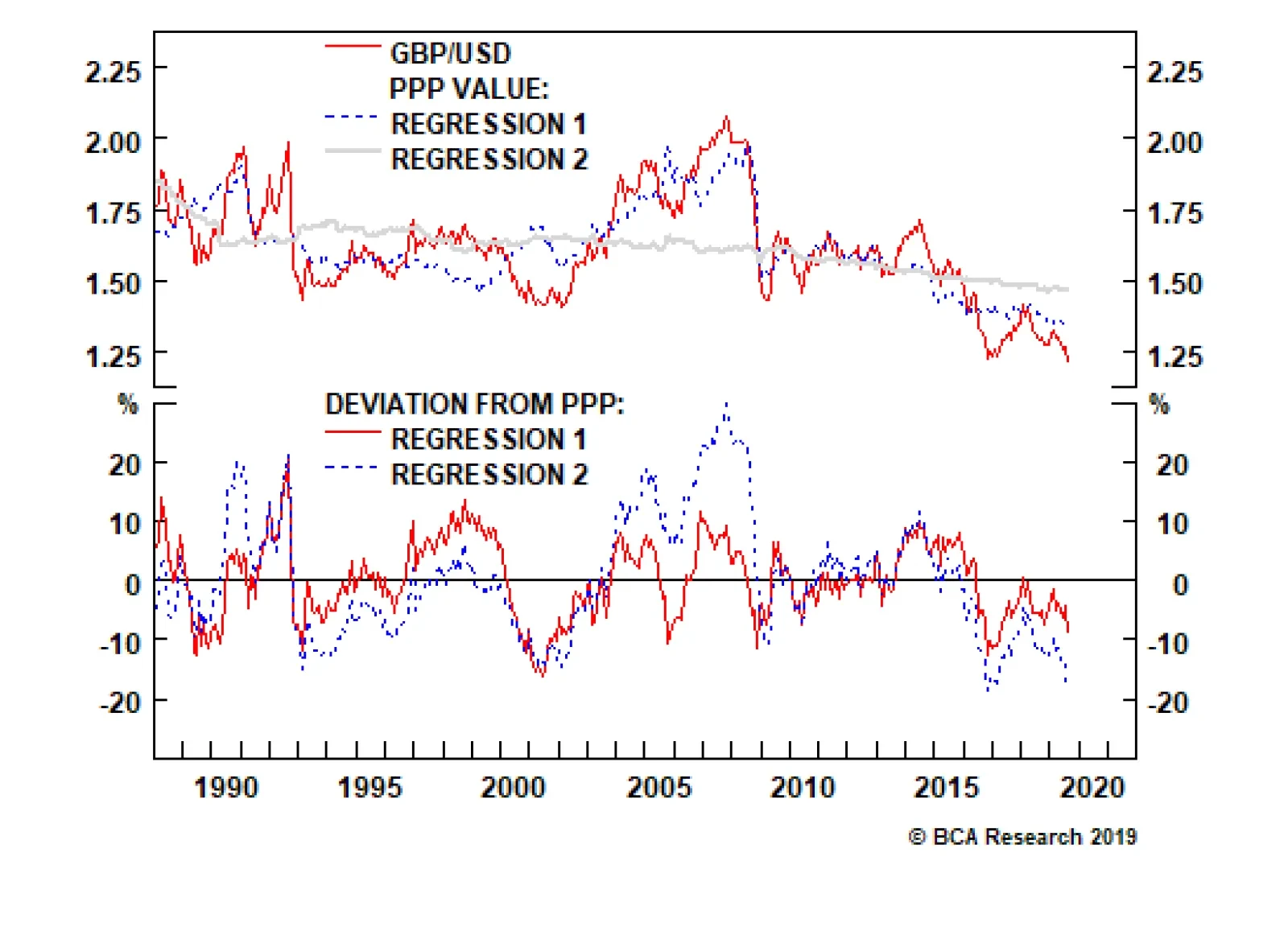
Both our regression models show the pound as undervalued. This supports our view that over the long term, the pound is attractive. The consumption baskets in both the U.K. and the U.S. are roughly similar, which means traditional PPP models do a good job at…
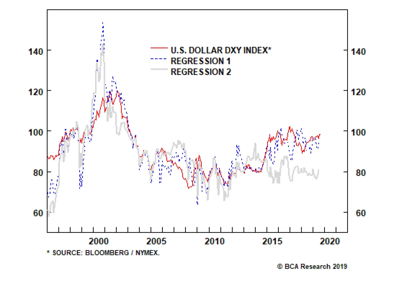
We reverse-engineered the fair value for the DXY index by aggregating the model results from its six constituents, using the corresponding DXY weights. This includes the euro, the Japanese yen, the British pound, the Canadian dollar, the Swedish krona, and…
Dear Client, Please note that there will be no regular Weekly Report next week, as we take a summer break. Our regular publication will resume September 6th. Best regards, Chester Ntonifor, Vice President Foreign Exchange Strategy Highlights Our PPP models show the DXY index to be overvalued by 10-15%. Within the G10 universe, the cheapest currencies are the Swedish krona, the British pound, the Japanese yen and the Norwegian krone. Look to go short CHF/GBP on valuation grounds. Feature Regular readers of our publication will notice that we tend to adhere to very simple and time-tested ideas. One such is the concept of purchasing power parity (PPP). The beauty comes from its simplicity. If the price of a good in Sweden is rising faster than in South Africa, then the krona should depreciate versus the rand to equalize prices across both borders. Otherwise, the krona becomes incrementally expensive, relative to the rand. In practice, various models have shown PPP to be a very poor tool for managing currencies. One roadblock comes from measurement issues, since consumer price baskets tend to differ in composition from one country to the next. Second, there is less price discovery for services, than there is for tradable goods. For example, it is rather difficult to import a haircut from Mumbai into the U.S., and so arbitraging those prices away tends to be impractical. Tariffs, trade restrictions and transport costs also tend to dampen the explanatory power of PPP models, though those have had diminishing importance over time. In order to get closer to an apples-to-apples comparison across countries, we make two adjustments. First, we divide the consumer price index (CPI) baskets into five major groups. In most cases, this breakdown captures 90% of the national CPI basket: Food, restaurants and hotels Shelter Health, culture and recreation Energy and transportation Household goods The second adjustment is to run two regressions with the exchange rate as the dependent variable. The first regression (call it REG1) uses the relative price ratios of the five groups as independent variables. This allows us to observe the most influential price ratios that help explain variations in the exchange rate. The second regression (call it REG2) uses a weighted average combination of the five groups to form a synthetic relative price ratio. If for example, shelter is 33% in the U.S. CPI basket, but 19% in the Swedish CPI basket, relative shelter prices will represent 26% of the combined price ratio. This allows for a uniform cross-sectional comparison, compared to using the national CPI weights. The results were largely consistent: Both regressions were statistically significant, but more so for REG1. This makes intuitive sense, as the number of variables were higher in the first regression. The sign for household goods was negative for some countries. This could be due to some specter of multicollinearity, if the tradable goods price effect is captured in other categories. There is also the low value-to-weight ratio for many household goods such as refrigerators or air conditioners, which could make currency deviations from PPP persistent. The shelter sign was also negative for some countries, meaning rising shelter prices tended to be associated with an incrementally cheaper currency. This could be due to the Balassa-Samuelson effect. Rising incomes (one key determinant of rising house prices) usually reflect rising productivity levels, which tend to lift the fair value of the exchange rate. The results showed the U.S. dollar as overvalued, especially versus the Swedish krona, British pound and Norwegian krone. Commodity currencies were closer to fair value, and within the safe haven complex, the Japanese yen was more attractive than the Swiss franc. The euro was less undervalued than implied by the overvaluation in the DXY index. As a final note, PPP models are just an additional kit to our currency toolbox, and so should never be used in isolation, but in conjunction with other currency signals. This is just a first iteration in our PPP modelling work, which we intend to improve in the months to come. U.S. Dollar We reverse-engineered the fair value for the DXY index by aggregating the model results from its six constituents. This includes the euro, the Japanese yen, the British pound, the Canadian dollar, the Swedish krona, and the Swiss franc, using the corresponding DXY weights. The message from the synthetic model is clear: the U.S dollar is above its fair value, in line with our fundamental view (Chart 1). Chart 1The Dollar is Slightly Expensive
The Dollar is Slightly Expensive
The Dollar is Slightly Expensive
Americans spent 35% of their income in 2018 on goods and 65% on services. Shelter remains the single largest consumption item for American households, which makes up 33% of the consumption basket. However, the relative importance of shelter is dwarfed by much more rampant rent and house price increases in other developed countries. Medical care accounts for 8.7% of the CPI basket, and is the highest in the developed world on a per capita basis. Total spending on health care accounts for almost 20% of nominal GDP. Since the 1980s, the CPI for medical care has risen fivefold, far outpacing many developed countries. This makes the dollar incrementally expensive. Core CPI edged higher to 2.2% in July, driven by medical care and shelter. While above the Federal Reserve’s 2% target, the risks to inflation remain asymmetric to the downside. That will keep the Fed on a dovish path near-term, which should help close overvaluation in the dollar. Euro We had limited data for the euro area, and so our regression results were less robust. REG1 shows the euro as cheap, while REG2 is more ambiguous (Chart 2). In short, a PPP model for the euro had one of lowest explanatory powers within the G10 universe. Food, restaurants and hotels are the largest consumption item in the euro CPI basket. Looking at the details, food and non-alcoholic beverages account for 14%, alcohol and tobacco make up 4%, and restaurant and hotels account for about 10% (Table). Relative price trends have moved to undermine the fair value of the euro. Chart 2The Euro Is Slightly Cheap
The Euro Is Slightly Cheap
The Euro Is Slightly Cheap
Euro Area CPI Weights
A Fresh Look At Purchasing Power Parity
A Fresh Look At Purchasing Power Parity
Shelter’s weight in the euro area CPI basket currently stands at 16.7%, the smallest among G10 countries. Since 2012, relative house and rent prices in the euro area have been decreasing compared with that in the U.S. Rampant rent controls, especially in places like Germany have subdued housing CPI, and tempered the fair value of the euro. This makes sense to the extent that it represents a concomitant rise in the welfare state. It is well-known that the euro area is relatively open and so tradable goods prices are important for the fair value of the euro. Given that the epicenter of trade tensions is between the U.S. and China, this will act to boost the relative attractiveness of European goods, which will be a bullish underpinning for the euro. Inflation expectations have collapsed in the euro area. However, compared to the Federal Reserve, there is little the European Central Bank can do to boost inflation. This is relatively euro bullish. Once global growth eventually picks up, improved competitiveness in the periphery will allow for non-inflationary growth. Japanese Yen The yen benefits from being cheap, as well as being a safe-haven currency (Chart 3). The overarching theme for Japan is a falling (and rapidly aging) population, which means that deficient demand and falling prices are the norm. This makes the yen relatively attractive on a recurring basis. Most of the Heisei era in Japan has been characterized by deflation. Importantly, all categories in Japan have been in a relative price downtrend during this period (Table). Domestically, an aging population (that tends to be a large voting base), prefer falling prices. Meanwhile, the bursting of the asset bubble in the late 80s/early 90s led to a powerful deleveraging wave that undermined prices. Chart 3The Yen Is Quite Cheap
The Yen Is Quite Cheap
The Yen Is Quite Cheap
Japan CPI Weights
A Fresh Look At Purchasing Power Parity
A Fresh Look At Purchasing Power Parity
The relative prices for most items have been decreasing, but culture and recreation inflation have experienced a meaningful rebound since 2013, largely due to a booming tourism industry in Japan.1 According to tourism statistics, the number of international visitors to Japan reached 31 million in 2018, almost five times the number ten years ago. But as long as the younger generation in Japan continues to save more and consume less, prices will remain under pressure. BoJ Governor Haruhiko Kuroda remains committed to achieving a 2% inflation target, but inflation expectations are falling to historical lows at a time when the BoJ is running out of policy bullets.2 That means inflation will likely lag that of other developed countries, lifting the fair value of the yen. British Pound Both regressions show the pound as undervalued. This supports our view that over the long term, the pound is a categorical buy (Chart 4). The consumption baskets in both the U.K. and the U.S. are roughly similar, which means traditional PPP models do a good job at capturing the true underlying picture of price differentials (Table). For example, OECD PPP models, based on national expenditure, show the pound as 15% undervalued. Chart 4The Pound Is Cheap
The Pound Is Cheap
The Pound Is Cheap
U.K. CPI Weights
A Fresh Look At Purchasing Power Parity
A Fresh Look At Purchasing Power Parity
Housing is the largest item in the consumption basket, with a total weight close to 30% (including housing electricity and water supply). The shelter consumer price index in the U.K. started to fall relative to the U.S. in 2016, which has lowered the fair-value of the pound (in the Balassa-Samuelson framework). That said, the fall in the pound has been much more deep and violent than suggested by domestic price fundamentals. For example, food restaurants and hotels are 10% cheaper in the U.K. compared to the U.S. over the last half decade. However, rather than appreciating 10%, the pound has plummeted by about 30%. Brexit will continue to dictate the ebb and flow of sterling gyrations, but the reality is that the pound should be higher on a fundamental basis. Meanwhile, a pick up in the global economy will benefit the pound. Going short CHF/GBP on valuation grounds is an attractive bet today. Australian Dollar As a commodity currency, PPP models are less useful for the Australian dollar than terms of trade, or even interest rate differentials. That said, the Aussie dollar is still relatively cheap versus the USD on a PPP basis (Chart 5). The key driver for value in the AUD has been a drop in the currency, relative to what price differentials will dictate. Food, restaurants and hotels comprise 23% of the Australian CPI basket, with the alcohol and tobacco category alone making up 7.4% (Table). Given food price differentials have been stable versus the U.S. in over a decade, Aussie citizens have not been particularly worse off. Chart 5The Aussie Is Slightly Cheap
The Aussie Is Slightly Cheap
The Aussie Is Slightly Cheap
Australia CPI Weights
A Fresh Look At Purchasing Power Parity
A Fresh Look At Purchasing Power Parity
Shelter accounts for almost a quarter percent of the basket. Relative shelter prices in Australia have been rising since the late 1990s, but started to soften in the past few years, on the back of macro prudential measures. Meanwhile, holiday travel and accommodation have a total weight of 6%, of which domestic travel makes up 2.9%, and international travel 3.1%. The overall cost of tourism in Australia has been falling relative to the U.S., boosting the fair value of the Aussie. In the 1980s, inflation in Australia averaged around 8.3% year-on-year. This made the Aussie incrementally expensive, creating grounds for a subsequent 50% devaluation from 1980 to 1986. Inflation targeting was finally introduced and has realigned Aussie prices with the rest of the world. Our bias is that the Aussie will be less driven by price differentials going forward, but more by RBA policy and terms of trade. New Zealand Dollar The New Zealand dollar is at fair value according to both models (Chart 6). Like the aussie, the kiwi is less driven by price differentials and more by terms of trade. Food and shelter account for the largest share of the consumption basket, and relative prices have not been moving in favor of the kiwi (Table). So, while the kiwi was overvalued earlier this decade, the overvaluation gap has been mostly closed via a higher dollar. Chart 6The Kiwi Is At Fair Value
The Kiwi Is At Fair Value
The Kiwi Is At Fair Value
New Zealand CPI Weights
A Fresh Look At Purchasing Power Parity
A Fresh Look At Purchasing Power Parity
Relative shelter prices in New Zealand have been soaring in recent decades compared to the U.S. Higher immigration, foreign purchases and a commodity boom helped. However, in August 2018, the ban on foreign property purchases came into effect, which helped cool down the housing market. Like in Australia, the inflation rate in New Zealand reached 18% year-on-year in the early 1980s, and was subsequently addressed via inflation targeting. This has realigned New Zealand prices somewhat with the rest of the world. Our bias is that going forward, the kiwi will underperform the aussie, mainly because of a negative terms of trade shock. Canadian Dollar The loonie is currently trading below its fair value, according to both of our models (Chart 7). Shelter remains the largest budget item for Canadian households (Table). The average Canadian household spent C$18,637 on shelter per year, around 29.2% of the total consumption in 2017.3 Interestingly, the shelter consumer price index does not fully capture skyrocketing house prices in Canada over the last decade. Since 2005, Canadian house prices relative to U.S. have doubled, according to OECD. On the contrary, the relative shelter CPI has trended downwards. These crosscurrents have dampened the explanatory power of the exchange rate. Chart 7The Loonie Is Slightly Cheap
The Loonie Is Slightly Cheap
The Loonie Is Slightly Cheap
Canada CPI Weights
A Fresh Look At Purchasing Power Parity
A Fresh Look At Purchasing Power Parity
Canadians are avid users of private transportation. The average spending on transportation accounted for 20% of total consumption, the second-largest expenditure item. Relative prices in this category have been rising, which has lowered the fair value of the exchange rate. Canada stands as the sixth largest energy producer in the world, but due to heavy taxation, Canadian consumers are paying more for gas prices than their U.S. neighbors. That said, terms of trade have been more important than PPP concerns for the loonie. In the near term, we believe energy prices (and the Western Canadian Select price spread) will continue to be important for the loonie. Swiss Franc USD/CHF is trading slightly below fair value, despite structural appreciation in the franc in recent years (Chart 8). The largest consumption item in Switzerland is the food, restaurants and hotels category (Table). The second item is shelter. Social services have a higher weight in the CPI basket, compared to other developed nations. This has been a huge driver of relative prices between Switzerland and the rest of the world, with falling relative prices boosting the fair value of the franc. Chart 8The Swiss Franc Is At Fair Value
The Swiss Franc Is At Fair Value
The Swiss Franc Is At Fair Value
Switzerland CPI Weights
A Fresh Look At Purchasing Power Parity
A Fresh Look At Purchasing Power Parity
Healthcare notably accounts for 15.5% in the total CPI basket, of which patient services makes up 11.5%. The Swiss healthcare system is a combination of public, subsidized private, and entirely private systems. It is mandatory for a Swiss resident to purchase basic health insurance, which covers a range of treatments. The insured person then pays the insurance premium plus part of the treatment costs. Finally, as a small open economy, tradable goods prices are important for Switzerland. Given high levels of specialization, terms-of-trade in Switzerland are soaring to record highs. This makes the franc a core holding in a currency portfolio. Norwegian Krone The Norwegian krone is undervalued according to both models (Chart 9). Food and shelter account for the largest share of the Norwegian CPI basket (Table). While the share of shelter is lower than in the U.S., other categories share similar weights, allowing traditional PPP models to be adequate for USD/NOK. One difference is that in terms of social services, only 0.2% of the expenditures are allocated to education, since all schools are free in Norway, including universities. Chart 9The Norwegian Krone Is Cheap
The Norwegian Krone Is Cheap
The Norwegian Krone Is Cheap
Norway CPI Weights
A Fresh Look At Purchasing Power Parity
A Fresh Look At Purchasing Power Parity
As a large energy producer, Norwegians pay less for electricity, gas, and other fuels. Norway is also a heavy producer of renewable energy, notably hydropower. This makes the domestic energy basket less susceptible to the ebbs and flows of energy prices. Going forward, the path of energy prices will continue to dictate ebbs and flows in the krone. Meanwhile, long NOK positions also benefit from an attractive valuation starting point. Swedish Krona The krona is the cheapest currency in our universe by a wide margin (Chart 10). This stems less from fluctuations in relative prices and more from negative rates that have hammered the exchange rate. Like many countries, food and shelter is the largest component of the consumption basket (Table). Transportation is also important. However, an important driver for undervaluation in the currency has been a drop in the relative price of social services. Chart 10The Swedish Krona Is Very Cheap
The Swedish Krona Is Very Cheap
The Swedish Krona Is Very Cheap
Sweden CPI Weights
A Fresh Look At Purchasing Power Parity
A Fresh Look At Purchasing Power Parity
Sweden experienced very high inflation rates in the 1980s, and since then, has been in a disinflationary regime. More recently, the inflation rate has edged down below the Riksbank’s target, mostly dragged down by recreation, culture, and healthcare. This makes Swedish real rates relatively attractive. We remain positive on the Swedish krona and believe that it will be one of the first to benefit, should global growth pick up. Chester Ntonifor, Foreign Exchange Strategist chestern@bcaresearch.com Kelly Zhong, Research Analyst kellyz@bcaresearch.com Footnotes 1 We removed the shelter component in regression 1, since it was distorting results. 2 Please see Foreign Exchange Strategy Weekly Report, titled “Short USD/JPY: Heads I Win, Tails I Don’t Lose Too Much”, dated May 31, 2019, available at fes.bcaresearch.com 3 Please see “Survey of Household Spending, 2017,” Statistic Canada, December 12, 2018. Trades & Forecasts Forecast Summary Core Portfolio Tactical Trades Limit Orders Closed Trades
Hard-to-predict policy risks and trade-war uncertainty will continue to hinder oil-demand growth, as will USD strength. The cost of oil in local-currency terms remains close to highs not seen since Brent and WTI traded above $100/bbl in 2014 in key EM economies, which partly explains the fall-off in demand begun in 2H18 that carried into 1H19 (Chart of the Week). We continue to expect oil demand to revive on the back of global fiscal and monetary stimulus, which, along with continued production discipline by OPEC 2.0 and capital discipline by U.S. shale producers, keeps our 2020 Brent forecast at $75/bbl. For 2019, however, our Brent forecast falls to $66/bbl from $70/bbl, following a re-basing of estimated demand in 2017-18 to bring it in line with lower historical data, and the lingering impact of a stronger USD.1 We also are revising our WTI expectation, as markets price in the last bits of ~ 2mm b/d of new pipeline takeaway capacity coming online in the Permian Basin. For 2019, we expect WTI to trade $6.50/bbl under Brent, and $4/bbl under next year, vs. $7/bbl and $5/bbl we expected last month. Chart of the WeekUSD Strength Hinders Oil-Demand Rebound
USD Strength Hinders Oil-Demand Rebound
USD Strength Hinders Oil-Demand Rebound
Highlights Energy: Overweight. Distillate fuel accounted for 29.6% of the product derived from refining crude oil in the U.S. during July, a record for the month, according to the Energy Information Administration (EIA). Refiners are gearing up for the global change-over to low-sulfur marine fuels ahead of the January 1, 2020, implementation of IMO 2020. Base Metals: Neutral. Increased infrastructure spending will add ~ $2 billion (14 billion RMB) to China’s total infrastructure spending of 524 billion RMB, according to a Fastmarkets MB analyst survey. Copper usage is expected to increase as 2H19 grid spending picks up. Precious Metals: Neutral. Gold and silver continue to mark time close to recent highs. USD strength could slow the metals’ rally. We remain long both metals as portfolio hedges. Ags/Softs: Underweight. This week’s USDA’s Crop Progress report showed 56% of the corn crop was in good or excellent condition, vs. 68% in 2018. For beans, 53% of the crop is in good or excellent condition, vs. 65% last year. Feature We expect global fiscal and monetary stimulus to lift demand in EM economies, which will be visible over the balance of this year and next. In this month’s assessment of supply-demand balances, we are lowering our 2019 Brent forecast to $66/bbl from $70/bbl, after re-basing our demand estimates so that they are more in line with EIA’s historical data (Chart 2). We lowered our historical demand estimates up to and including 2017, in line with the EIA data. This reduces the base level for 2018-20 demand. As a result, the level of our 2018 demand is down by 200k b/d to 100.1mm b/d, vs. last month’s estimate, and the level of our 2019 and 2020 demand estimates is down by 250k b/d to 101.3mm b/d and to 102.8mm b/d. The adjustments are mainly due to the revision of historical level of demand in 2017-2018. In addition, we lowered our growth estimate for 2019 slightly to 1.2mm b/d from 1.25mm b/d last month, but kept our 2020 growth rate expectation at 1.5mm b/d. Chart 2Lower 2019 Demand Estimate, Price; Keeping 2020 Unchanged
Lower 2019 Demand Estimate, Price; Keeping 2020 Unchanged
Lower 2019 Demand Estimate, Price; Keeping 2020 Unchanged
As noted above, we expect global fiscal and monetary stimulus to lift demand in EM economies, which will be visible over the balance of this year and next. Continued production discipline by OPEC 2.0 and capital discipline by U.S. shale producers leaves our 2020 Brent forecast unchanged at $75/bbl. In addition, this combination of stronger demand and tighter supply will create a physical supply deficit (Chart 3). This deficit will force inventories lower, which remains OPEC 2.0’s paramount goal, and backwardate the Brent and WTI forward curves (Chart 4). Chart 3Stronger Demand, Tighter Supply Produces Physical Deficit
Stronger Demand, Tighter Supply Produces Physical Deficit
Stronger Demand, Tighter Supply Produces Physical Deficit
Chart 4Inventory Draws Will Resume
Inventory Draws Will Resume
Inventory Draws Will Resume
For WTI, we now expect it to trade $6.50/bbl under Brent in 2019 and $4/bbl under in 2020, vs. the $7/bbl and $5/bbl differentials we expected last month. This narrowing of the differential comes on the back of the build-out of takeaway pipeline capacity in the Permian Basin, which amounts to ~ 2mm b/d by the end of this year. The expansion of deep-water harbor capacity in the U.S. Gulf is being delayed by regulatory action, which means the Brent vs. WTI differential will not significantly contract further until later in 2020 or 2021 when we expect crude-oil export volumes to pick up sharply. Over the course of the coming year, we do expect exports to pick up before 2021, as they have done in 2018-2019. This trend likely continues. We calculated there is ~ 4.5 mm b/d of current export capacity in the Gulf, therefore exports still can increase before being fully constrained. In addition, small capacity expansion projects already are under construction, which will lift capacity next year. That said, any delays could pressure differentials (LLS-Brent, WTI-Brent). But, as long as shale-oil production keeps increasing and foreign demand remains strong, exports can increase – likely at a slower pace – while differentials hold around the $4/bbl level next year. Digging Into The Oil Demand Slow-Down This was a stealthy USD rally, overshadowed by the Sino-U.S. trade war, and exogenous foreign-policy shocks re U.S. Venezuela and Iran policy. For 2019, a grouping of negative demand-side effects have proven to be quite strong – uncertainty spawned by the Sino-U.S. trade-war, tightening financial conditions globally, and the strong USD. Over the past year, these effects have combined to lower actual demand, and forced us to lower our growth expectation for this year for a fourth time to 1.2mm b/d. In hindsight, it is apparent the strong USD has affected EM demand by raising the local-currency cost of oil in particular over the past year to levels not seen since crude was trading above $100/bbl in 2014 (Charts 5A and 5B). Chart 5AAs USD Strengthened Local-Currency Costs Skyrocketed
As USD Strengthened Local-Currency Costs Skyrocketed
As USD Strengthened Local-Currency Costs Skyrocketed
Chart 5BAs USD Strengthened Local-Currency Costs Skyrocketed
As USD Strengthened Local-Currency Costs Skyrocketed
As USD Strengthened Local-Currency Costs Skyrocketed
This was a stealthy USD rally, overshadowed by the Sino-U.S. trade war, and exogenous foreign-policy shocks re U.S. Venezuela and Iran policy. In addition to raising the cost of commodities priced in USD, in local-currency terms, the stronger dollar lowered the cost of producing commodities for countries like Russia, whose currencies are not pegged to the USD. So, in one fell swoop, USD strength lowered demand via higher prices, and increased supply via lower costs of production. In addition, weaker local currencies catalyze capital outflow, which reduces the supply of savings available to EM economies for investment. At the margin, this also stunts income growth.2 The effects of USD strength could persist, and continue to have a deleterious influence on oil demand into next year, given the way in which monetary policy – and its effects on FX rates – can act with “long and variable lags.” Our BCA Commodity-Demand Nowcasting model continues to point toward a revival of demand as EM economic growth picks up (Chart 6).3 Given the dollar is a counter-cyclical currency vis-à-vis the rest of the world, we expect this will weaken the USD and be supportive of commodity prices. Chart 6BCA Commodity-Demand Nowcast Remains Upbeat
BCA Commodity-Demand Nowcast Remains Upbeat
BCA Commodity-Demand Nowcast Remains Upbeat
Chart 7Expect Further Backwardation In Crude Oil Forward Curves
Expect Further Backwardation In Crude Oil Forward Curves
Expect Further Backwardation In Crude Oil Forward Curves
Higher oil demand and lower supply likely will further backwardate Brent and WTI forward curves, which will diminish the impact of the USD’s strength (Chart 7), and lead to higher volatility, as fundamentals once again dominate price formation (Chart 8). Still, the effects of USD strength could persist, and continue to have a deleterious influence on oil demand into next year, given the way in which monetary policy – and its effects on FX rates – can act with “long and variable lags," to borrow Milton Friedman's well-turned phrase.4 We will monitor this risk closely, and will be offering further research into it.
Chart 8
Supply Concerns Persist E&P companies are using their accumulated inventory of excess Drilled-but-Uncompleted (DUC) wells to reach their production targets, while controlling capital expenditures (i.e. flat/lower rig count). We continue to expect OPEC 2.0 to manage production, and to keep a laser focus on reducing inventories. The producer coalition continues to get a huge assist in this effort from the U.S. sanctions against Iran, which, according to the American Secretary of State Mike Pompeo have taken almost all of that country’s oil exports – some 2.7mm b/d – out of the market (Chart 9).5
Chart 9
In our balances estimates, we show OPEC producing 29.8mm b/d of crude oil on average this year, and 29.7mm b/d next year. This is down sharply from the 32mm b/d we estimate the Cartel produced last year, which included a surge in 2H18 undertaken in response to pressure from the U.S. to build inventories ahead of oil-export sanctions being re-imposed against Iran (Table 1). Given the lower demand estimate OPEC is forecasting for this year and next – 99.9mm b/d, and 101.1mm b/d this year and next – we expect OPEC’s leader, KSA, to keep production closer to 10mm b/d vs. its 10.33mm b/d quota. We expect the other putative leader of OPEC 2.0, Russia, to produce 11.43mm b/d and 11.41mm b/d this year and next, versus 11.4mm b/d last year. Table 1BCA Global Oil Supply - Demand Balances (MMb/d, Base Case Balances)
USD Strength Slows Oil Demand Growth; 2020 Brent Forecast Remains At $75/bbl
USD Strength Slows Oil Demand Growth; 2020 Brent Forecast Remains At $75/bbl
Once again, U.S. shale-oil output provides the largest increase in supply globally. That said, shale-oil producers are being forced to temper production growth, as investors’ demand higher profits or greater return of capital. We revised down our U.S. shale production growth to 8.2mm b/d in 2019 and 9.1mm b/d in 2020 (Chart 10). In 2018, we estimated U.S. shale production at 7.2mm b/d. Chart 10Shale Output Reduced Slightly
Shale Output Reduced Slightly
Shale Output Reduced Slightly
Chart 11
Lower-than-expected WTI prices and capital discipline will limit U.S. shale production growth this year, and temper it next year. E&P companies are using their accumulated inventory of excess Drilled-but-Uncompleted (DUC) wells to reach their production targets, while controlling capital expenditures (i.e. flat/lower rig count).6 Year to date, DUC completions increased in the Big Five tight-oil basins, overtaking new wells drilled (Chart 11).7 However, the Permian’s excess DUC inventory increased in July despite the ongoing pipeline capacity expansion and falling rig count. The Permian’s completion rate will be important to monitor. At current oil prices, producers need to tap into their excess DUC inventories to reach both their free-cash-flow and production goals. Bottom Line: We are reducing our Brent price forecast for 2019 to $66/bbl, on the back of weaker demand. Our forecast for 2020 remains unchanged at $75/bbl. Our expectations are driven by our expectation fiscal and monetary stimulus to lift commodity demand – oil in particular – and that production discipline by OPEC 2.0 and capital discipline from U.S. shale-oil producers will tighten markets and lift prices from here. Robert P. Ryan, Chief Commodity & Energy Strategist rryan@bcaresearch.com Hugo Bélanger, Senior Analyst Commodity & Energy Strategy HugoB@bcaresearch.com Footnotes 1 OPEC 2.0 is the name we coined for the producer coalition formed in late 2016 by the Kingdom of Saudi Arabia (KSA) and Russia. The producer coalition’s mission was – and remains – managing global supply so as to reduce inventories. We expect OPEC 2.0 production to be at or below quota levels agreed December 7, 2018, when KSA and Russia and their respective allies set about once again to drain global inventories of the 62-million-barrel overhang that resulted from the production ramp-up undertaken in response to demands from U.S. President Donald Trump. 2 The International Energy Agency (IEA) noted that, on the back of higher prices last year, oil once again was “the most heavily subsidized” energy source, expanding its share of the $400 billion provided consumers by their governments to 40%. Please see Commentary: Fossil fuel consumption subsidies bounced back strongly in 2018, published by the IEA June 13, 2019. 3 For a description of our nowcast model, please see Just In Time For Christmas! U.S. Tariff Delay Rocks Oil published last week by BCA Research’s Commodity & Energy Strategy. It is available at ces.bcaresearch.com. We noted last week that our expectation of stronger EM growth and a weaker USD is contrary to the view of BCA Research’s Emerging Markets Strategy, which expects continued weakness in EM GDP growth. Moreover, as mentioned in last week's report, our nowcast’s last data point was observed in July, which is before the latest escalation in trade tensions. We could see a move down in some of the indicators used as input in our nowcast model in the coming month. 4 Friedman, the 1976 Nobel Laureate in Economics, noted monetary policy operates with long and varying lags, which makes it difficult to be precise as to when its effects will be noticed in the macroeconomy. Please see Milton Friedman’s article, “The Lag in Effect of Monetary Policy,” Journal of Political Economy Vol. 69, No. 5 (Oct., 1961), pp. 447-466. 5 To date, OPEC and non-OPEC producers have had no apparent trouble replacing lost Iranian and Venezuelan barrels taken off the market as a result of U.S. sanctions. This indicates spare capacity remains sufficient to meet short-term supply disruptions and unplanned outages. Please see U.S. removed almost 2.7 million barrels of Iranian oil from market - Pompeo, published by uk.reuters.com August 20, 2019. 6 The process of drilling and completing wells produces a normal inventory of uncompleted wells, because of the time lag between the moment wells are drilled and the time they are completed. The development of multi-well pad drilling in U.S. shales structurally increased the time lag between drilling and completion to ~ 5 months. This implies a normal level of DUC inventory that corresponds to ~ 5 - 6 months’ worth of drilling activity. We define any DUC above our estimate of normal as an excess DUC well. On average, completion accounts for ~ 65% of the total well costs. 7 The Big Five shale basins are the Permian; the Eagle Ford; Niobrara; the Bakken, and the Anadarko. Investment Views and Themes Recommendations Strategic Recommendations Tactical Trades TRADE RECOMMENDATION PERFORMANCE IN 2019 Q2
Image
Commodity Prices and Plays Reference Table Trades Closed in 2019 Summary of Closed Trades
Image
Highlights Duration: Global manufacturing growth will rebound near the end of this year. Much like in 2016, this will result in higher global bond yields on a 12-month horizon. Investors should keep portfolio duration close to benchmark for now, but be prepared to shift to below-benchmark when our global growth indicators show signs of improvement. Country Allocation: Countries with yield curves furthest away from the effective lower bound also have the most cyclical bond markets. At present, this means that U.S. and Canadian bond markets will perform best if global growth continues to weaken. They will also perform worst in the event of an economic turnaround. Japanese bonds will perform best in a bond bear market, with German debt a close second. Relative Value In Global Government Debt: Changes in the level and shape of global yield curves have altered the relative value opportunities in the global government bond space. We find that the most positive carry (including both yield income and rolldown) in global government bond markets is earned in 30-year German, Japanese and Australian bonds, and in 10-year U.K. and Japanese bonds. Feature Reflexivity Chart 1A Brief Inversion
A Brief Inversion
A Brief Inversion
The decline in global bond yields has been unrelenting, and it took on a life of its own last week when the U.S. 2-year/10-year slope briefly inverted (Chart 1). After the inversion, the 30-year U.S. Treasury yield broke below 2% and the 10-year yield broke below 1.50%. The average yield on the 7-10 year Global Treasury Index closed at 0.49% last Thursday, just above its all-time low of 0.48% (Chart 1, bottom panel). There’s an interesting self-fulfilling prophesy that can take hold when the yield curve inverts. Investors interpret the inversion as a signal of weaker economic growth ahead. They then bid up long-dated bond prices causing the curve to invert even more. This sort of circular reasoning can cause bond yields to disconnect from the trends in global economic data, often severely. While recession fears have benefited government bonds, risky assets – equities and corporate bonds – have experienced relatively minor pain. The S&P 500’s recent sell-off pales in comparison to the one seen late last year (Chart 2). Meanwhile, corporate bond spreads remain well below early-2019 peaks. Risky assets have clearly benefited from the drop in bond yields, as markets price-in a future where central banks ease monetary policy in response to weaker economic growth, and where that easing is sufficient to keep equities and credit well supported. Chart 2Low Yields Support Risk Assets I
Low Yields Support Risk Assets I
Low Yields Support Risk Assets I
Chart 3Low Yields Support Risk Assets II
Low Yields Support Risk Assets II
Low Yields Support Risk Assets II
Further evidence of this dynamic is presented in Chart 3. The chart shows the sensitivity of daily changes in the U.S. 10-year Treasury yield to changes in the S&P 500 for each year since 2010. The sample is split into days when the S&P 500 rose and when it fell. For example, in 2010 the sensitivity on “up days” was 2.6, meaning that on days when the S&P 500 rose, the 10-year yield rose 2.6 basis points for every 1% increase in the S&P 500. Similarly, the sensitivity in 2010 on “down days” was 3.2. This means that the 10-year yield fell 3.2 bps for every 1% drop in the equity index. The main takeaway from Chart 3 is how dramatically the sensitivities have shifted in 2019. The yield sensitivity on “up days” has fallen sharply – down to 0.8. This means that yields barely rise on days when equities move up. Meanwhile, the sensitivity on “down days” has shot higher, to just under 4. This means that yields fall a lot on days when equities sell off. The perception of easier monetary policy has been the main support for risk assets this year. The logical interpretation of these trends is that the perception of easier monetary policy has been the main support for risk assets this year. Global Growth Needed At present, we are stuck in an environment where aggressively easy monetary policy and low bond yields are the sole supports for risky assets. In turn, falling bond yields are stoking concerns about the economy, leading to even easier monetary policy. Only one thing can bust us out of this pattern, and that’s a resurgence of global manufacturing growth. Unfortunately, there is little evidence that this is taking place (Chart 4). The Global Manufacturing PMI is now down to 49.3, below the 2016 trough of 49.9 (Chart 4, top panel). U.S. Industrial Production growth remains weak, but is showing signs of stabilization above the 2016 trough (Chart 4, panel 2). European Industrial Production, on the other hand, continues to contract (Chart 4, panel 3). The downtrend in our favorite real-time indicator of global manufacturing – the CRB Raw Industrials index – remains unbroken (Chart 4, bottom panel). However, even though evidence of a turnaround in global manufacturing is scant, we expect a rebound near the end of this year, for the following reasons: Global financial conditions have eased this year, the result of aggressive central bank stimulus. Financial conditions are easier now than they were in 2018, and much easier than they were prior to the 2015/16 global growth slowdown (Chart 5, top panel). China has started to ease credit conditions in response to U.S. tariffs and the slowdown in growth. So far, stimulus has been tepid relative to 2015/16 levels, but it should ramp up in the coming months.1 Many large important segments of the global economy remain unaffected by the global manufacturing slowdown. The U.S. consumer continues to spend: Core retail sales are growing at a robust 5% year-over-year rate, and consumer sentiment remains elevated (Chart 5, panels 2 & 3). Even in the Eurozone, the service sector has not experienced the same pain as manufacturing (Chart 5, bottom panel). Fiscal policy will remain a tailwind for economic growth this year and next. Last week, there were even rumors of increased fiscal thrust from Germany if the growth slowdown persists.2 Strong inflation readings only increased market worries that the Fed might not be as accommodative as necessary. On the whole, we expect that the above 4 factors will lead to a rebound in global manufacturing growth near the end of this year. Much like in 2016, this will result in higher global bond yields on a 12-month horizon, but the global growth indicators shown in Chart 4 will need to rebound first. Chart 4Global Growth Indicators
Global Growth Indicators
Global Growth Indicators
Chart 5Catalysts For Economic Recovery
Catalysts For Economic Recovery
Catalysts For Economic Recovery
Inflation Puts Pressure On Powell Chart 6Strong Inflation Could Complicate The Fed's Message
Strong Inflation Could Complicate The Fed's Message
Strong Inflation Could Complicate The Fed's Message
Strong U.S. inflation prints during the past two months add an interesting wrinkle to the macro landscape. Core U.S. inflation grew at an annualized rate of 3.55% in July, following an annualized rate of 3.59% in June (Chart 6). However, these strong inflation readings only increased market worries that the Fed might not be as accommodative as necessary. This exacerbated the flattening of the yield curve and sent long-dated TIPS breakeven inflation rates lower. Our sense is that the Fed is chiefly concerned with re-anchoring inflation expectations (Chart 6, bottom panel). This probably means that another rate cut is coming in September, and that Chairman Powell will do his best to sound accommodative in his Jackson Hole address on Friday. However, recent strong inflation data could prompt Powell to sound more hawkish than the market would like, causing yield curves to flatten and risky assets to fall. Bottom Line: Global manufacturing growth will rebound near the end of this year. Much like in 2016, this will result in higher global bond yields on a 12-month horizon. Investors should keep portfolio duration close to benchmark for now, but be prepared to shift to below-benchmark when our global growth indicators show signs of improvement. Country Allocation & The Zero Lower Bound Perhaps the most straightforward way to think about country allocation within a portfolio of developed market government bonds is to classify the different markets as either “high beta” or “low beta”. Chart 7 shows the trailing 3-year sensitivity of major countries’ 7-10 year bond yields relative to the global 7-10 year yield.3 The U.S. and Canada have the highest betas, followed by the U.K. and Australia. Germany has a beta close to one, and Japan’s beta is the lowest. Chart 7Global Yield Beta
Global Yield Beta
Global Yield Beta
In other words, if global growth falters and global bond yields decline, U.S. and Canadian bond markets should perform best, followed by the U.K. and Australia. German bonds should perform in line with the global index, and Japanese bonds should underperform the global benchmark. What makes this approach to portfolio allocation even better is that the calculation of trailing betas is not really necessary. A very similar ordering of countries – from “high beta” to “low beta” – is achieved by simply ranking the markets from highest yielding to lowest yielding. High yielding countries, like the U.S. and Canada, have the most room to ease monetary policy in response to a negative growth shock. This means that yields in those countries will respond most to global growth fluctuations. On the other hand, the entire Japanese yield curve is already pinned near the effective lower bound. Even in the event of a negative growth shock, there is little scope for easier Japanese monetary policy, and JGB yields will be relatively unaffected. Chart 8High Beta Countries Are Most Sensitive To Economic Growth
High Beta Countries Are Most Sensitive To Economic Growth
High Beta Countries Are Most Sensitive To Economic Growth
It’s interesting to note in Chart 7 that while German yields are actually below JGB yields, bunds remain somewhat less defensive than the Japanese market. This is because the German term structure has only recently moved to the effective lower bound, and investors likely still retain some hope that an improvement in global growth could lead to European policy tightening at some point in the future. This belief is largely absent in Japan, where the term structure has been pinned at the lower bound for many years. Chart 8 provides some further evidence of the split between “high beta” and “low beta” bond markets. It shows that the bond markets with the highest yields are also the most sensitive to trends in global growth, as proxied by the Global Manufacturing PMI. U.S. bond yields are highly correlated with the Global PMI, while Japanese bond yields are hardly correlated at all. It follows that if the slowdown in global growth continues and all nations’ yield curves converge to Japanese levels, then the overall economic sensitivity of global bond yields will decline. Bottom Line: Countries with yield curves furthest away from the effective lower bound also have the most cyclical bond markets. At present, this means that U.S. and Canadian bond markets will perform best if global growth continues to weaken. They will also perform worst in the event of an economic turnaround. Japanese bonds will perform best in a bond bear market, with German debt a close second. Looking For Positive Carry Yield curves have undergone dramatic shifts in recent months, in terms of both level and shape. Not only have curves for the major government bond markets shifted down since the beginning of the year, they also now exhibit varying degrees of a ‘U’ shape (Charts 9A-9F). With that in mind, in this week’s report we look for the best “positive carry” opportunities in global government bond markets. Yield curves for the major government bond markets have shifted down since the beginning of the year, they also now exhibit varying degrees of a ‘U’ shape. We use the term carry to mean the expected return from a given bond assuming an unchanged yield curve. This is essentially the combination of yield income (i.e. coupon return) and the price impact of rolling down (or up) the yield curve. For the purposes of this report, we assume a 12-month investment horizon and incorporate the impact of currency hedging into each security’s yield income.
Chart 9
Chart 9
Chart 9
Chart 9
Chart 9
Chart 9
Rolldown ‘U’ shaped yield curves mean that bonds near the base of the ‘U’ currently suffer from negative rolldown, while the rolldown for long maturities is often highly positive. Table 1 shows that rolldown is currently negative for all 2-year bonds, but especially for U.S. and Canadian debt. The U.S. and Canada have the highest policy rates within developed markets, so it’s not surprising that the front-end of their yield curves are also the most steeply inverted. In other words, their yield curves are pricing-in that they have more room to cut rates than other countries. Table 112-Month Rolldown* (%) For A Long Position In Government Bonds
Where's The Positive Carry In Bond Markets?
Where's The Positive Carry In Bond Markets?
In general, rolldown is relatively modest for most 5-year and 7-year maturities. The exceptions being German 5-year debt and Aussie 7-year debt, which benefit from 31 bps and 45 bps of positive rolldown, respectively. As mentioned above, rolldown is currently very positive for long maturity debt. In fact, a 10-year U.K. bond offers a whopping 85 bps of rolldown on a 12-month horizon. Yield Income & Overall Carry As mentioned above, rolldown is only one part of a bond’s carry. The other is the yield an investor earns over the course of the investment horizon – the yield income. Because we assume that investors hedge the currency impact of their bond positions, this yield income also depends on the native currency of the investor. Therefore, we show yield income and overall carry below from the perspective of investors in each of the major currency blocs (USD, EUR, JPY, GBP, CAD, AUD). USD Investors Being the global high yielder, USD investors benefit the most from currency hedging. That is, USD investors earn a lot of additional income on their currency hedges, making non-U.S. bonds look more attractive. Unsurprisingly, carry is most positive at the long-end of yield curves (Tables 2 & 3). Table 2In USD: 12-Month Yield Income* (%) For A Long Position In Government Bonds
Where's The Positive Carry In Bond Markets?
Where's The Positive Carry In Bond Markets?
Table 3In USD: 12-Month Carry (%) For A Long Position In Government Bonds
Where's The Positive Carry In Bond Markets?
Where's The Positive Carry In Bond Markets?
EUR Investors The polar opposite of USD investors, EUR-based investors give up a lot of return through currency hedging. This makes the potential for positive carry much less. In any case, the best positive carry opportunities still lie in German, Japanese and Australian 30-year bonds. U.K. and Japanese 10-year bonds are also attractive (Tables 4 & 5). Table 4In EUR: 12-Month Yield Income* (%) For A Long Position In Government Bonds
Where's The Positive Carry In Bond Markets?
Where's The Positive Carry In Bond Markets?
Table 5In EUR: 12-Month Carry (%) For A Long Position In Government Bonds
Where's The Positive Carry In Bond Markets?
Where's The Positive Carry In Bond Markets?
JPY Investors Yen-based investors currently have more opportunities to earn positive carry than those based in euros. But these opportunities remain confined to long-maturity debt. Once again, the standouts are Japanese, German and Australian 30-year bonds, and also U.K. and Japanese 10-year debt (Tables 6 & 7). Table 6In JPY: 12-Month Yield Income* (%) For A Long Position In Government Bonds
Where's The Positive Carry In Bond Markets?
Where's The Positive Carry In Bond Markets?
Table 7In JPY: 12-Month Carry (%) For A Long Position In Government Bonds
Where's The Positive Carry In Bond Markets?
Where's The Positive Carry In Bond Markets?
GBP Investors Currency hedges work more in favor of GBP than EUR or JPY. As a result, GBP-based investors see more opportunities to earn positive carry (Tables 8 & 9). Table 8In GBP: 12-Month Yield Income* (%) For A Long Position In Government Bonds
Where's The Positive Carry In Bond Markets?
Where's The Positive Carry In Bond Markets?
Table 9In GBP: 12-Month Carry (%) For A Long Position In Government Bonds
Where's The Positive Carry In Bond Markets?
Where's The Positive Carry In Bond Markets?
CAD Investors As with USD-based investors, CAD-based investors also benefit from currency hedging. All securities continue to offer positive carry when hedged into CAD (Tables 10 & 11). Table 10In CAD: 12-Month Yield Income* (%) For A Long Position In Government Bonds
Where's The Positive Carry In Bond Markets?
Where's The Positive Carry In Bond Markets?
Table 11In CAD: 12-Month Carry (%) For A Long Position In Government Bonds
Where's The Positive Carry In Bond Markets?
Where's The Positive Carry In Bond Markets?
AUD Investors AUD-based investors also see positive carry across the entire global bond space, after factoring-in the impact of currency hedging (Tables 12 & 13). Table 12In AUD: 12-Month Yield Income* (%) For A Long Position In Government Bond
Where's The Positive Carry In Bond Markets?
Where's The Positive Carry In Bond Markets?
Table 13In AUD: 12-Month Carry (%) For A Long Position In Government Bonds
Where's The Positive Carry In Bond Markets?
Where's The Positive Carry In Bond Markets?
Bottom Line: Changes in the level and shape of global yield curves have altered the relative value opportunities in the global government bond space. We find that the most positive carry (including both yield income and rolldown) in global government bond markets is earned in 30-year German, Japanese and Australian bonds, and in 10-year U.K. and Japanese bonds. Ryan Swift, U.S. Bond Strategist rswift@bcaresearch.com Footnotes 1 Please see U.S. Bond Strategy Weekly Report, “The Trump Interruption”, dated August 13, 2019, available at usbs.bcaresearch.com 2 https://www.bloomberg.com/news/articles/2019-08-16/germany-ready-to-raise-debt-if-recession-hits-spiegel-reports 3 We calculate betas using average yields from the Bloomberg Barclays Global Treasury Master index. Fixed Income Sector Performance Recommended Portfolio Specification
However, things began to shift a few years ago. Following cascading crises (in Europe, Japan and even some commodity-producing countries, for example), interest rates outside the U.S. began to fall rapidly, and the U.S. bond market became one of the most…
It is too early to tell if the dollar’s muted response is just the lagged effect of thin summer trading, or a signal towards much bigger opposing forces at play. What we can infer is that both short-term and longer-term investors are caught in a stalemate. …