Labor Market

Highlights The Fed: The Fed will formally discuss tapering plans over the course of this summer and fall and announce the slowing of asset purchases before the end of 2021. Its labor market objectives will also be achieved in time to lift rates in 2022. Non-US Developed Markets: The central banks outside the US most likely to deliver tapering and/or outright rate hikes over the next 1-2 years are those facing housing bubbles – the Bank of Canada and Reserve Bank of New Zealand. The ECB will do nothing on rates while adjusting asset purchase programs to preserve the size of its balance sheet, while the Reserve Bank of Australia will also sit on their hands for longer. Bond Strategy Recommendations: Investors should maintain below-benchmark portfolio duration in US-only and global fixed income portfolios. Global bond investors should also favor exposure in markets where central banks will be more dovish than expected (core Europe, Australia), while limiting exposure to markets where hawkish surprises are more likely (the US, Canada, New Zealand). Feature The recovery from the 2020 COVID recession is now well underway and many investors are getting antsy about when central bankers might respond by removing monetary policy accommodation. Some central banks appear more eager than others. Both the Bank of Canada and Bank of England, for instance, have already started to reduce their rates of bond buying. Meanwhile, the US Federal Reserve is only just now starting to talk about the timing of its own tapering. This Special Report lays out a timeline for what central bank actions we should expect during the next two years. The first section focuses exclusively on the US Federal Reserve and the second section incorporates likely announcements from other central banks. Based on a comparison of our expected central bank timeline with current market prices, we conclude that investors should maintain below-benchmark portfolio duration in US-only and global fixed income portfolios. Global bond investors should also favor government bonds in countries where central banks are likely to be less hawkish than markets expect (core Europe, Australia) versus bonds from countries where hawkish surprises are more likely (US, Canada, New Zealand and, potentially, the UK and Sweden). The Federal Reserve’s Timeline Chart 1 shows our anticipated timeline for when the Federal Reserve will make specific policy announcements between now and the start of 2024. Chart 1The Federal Reserve’s Timeline
A Central Bank Timeline For The Next Two Years
A Central Bank Timeline For The Next Two Years
First, over the course of this summer, the Fed will initiate discussions about when to taper its asset purchases. Then, asset purchase tapering will be announced at the December 2021 FOMC meeting with purchases set to decline as of the beginning of 2022. We expect that net Fed purchases will fall to zero by the end of Q3 2022. That is, by that time the Fed will no longer be adding to its securities holdings. Rather, it will keep the size of its balance sheet constant. Then, with its balance sheet no longer growing, the Fed will begin the process of lifting interest rates. We expect the first rate hike to occur at the December 2022 FOMC meeting. Finally, some time after the fed funds rate is well above the zero bound, the Fed will try to reduce the size of its securities portfolio. How do we arrive at this timeline? Table 1A Checklist For Liftoff
A Central Bank Timeline For The Next Two Years
A Central Bank Timeline For The Next Two Years
We start with the Fed’s forward guidance about the timing of the first rate hike (Table 1). The Fed has told us that it will lift rates off the zero bound once (i) PCE inflation is above 2%, (ii) the labor market is at “maximum employment” and (iii) inflation is expected to remain above 2% for some time. The first item on the Fed’s liftoff checklist has already been met and the third item logically follows from the other two. That is, if inflation is above 2% and the labor market is at “maximum employment” then the Fed will certainly expect inflation to remain high. This means that the second item on the Fed’s checklist is the most critical for assessing the timing of liftoff. In assessing the US labor market’s progress toward “maximum employment” we first have to define what “maximum employment” means. Based on the Fed’s communications, we infer that “maximum employment” means an unemployment rate between 3.5% and 4.5% - a range consistent with the Fed’s NAIRU estimates – and a labor force participation rate that has recovered back to pre-pandemic levels (Chart 2). Table 2 presents the average monthly growth in nonfarm payrolls that is required to reach that definition of maximum employment by specific future dates. For example, we calculate that average monthly payroll growth of 698k to 830k will cause the labor market to reach maximum employment by the end of this year. Average monthly payroll growth of 412k to 493k is required to hit the Fed’s target by the end of 2022. Chart 2Defining "Maximum Employment"
Defining "Maximum Employment"
Defining "Maximum Employment"
Table 2Average Monthly Nonfarm Payroll Growth Required To Reach Maximum Employment By The Given Date
A Central Bank Timeline For The Next Two Years
A Central Bank Timeline For The Next Two Years
The most recent issue of the Bank Credit Analyst posits several reasons why US employment growth will pick up steam in the coming months.1 We agree with this view and note that indicators of labor demand such as job openings, the NFIB “jobs hard to get” survey and the Conference Board’s “jobs plentiful” survey also point to accelerating employment gains.2 All told, we think that average monthly payroll growth of 412k to 493k is eminently achievable (Chart 3). This means that the Fed will hit its three liftoff criteria in time to hike rates before the end of 2022. Chart 3Max Employment By The End of 2022
Max Employment By The End of 2022
Max Employment By The End of 2022
Working backwards from the expected liftoff date, the Fed has said that it needs to see “substantial progress” toward the criteria listed in Table 1 before it will taper its pace of asset purchases. The definition of “substantial progress” remains somewhat unclear, but a few recent Fed communications provide some clues. First, Fed Chair Jay Powell said that he wants to see a “string of months” like the strong March employment report before it will be appropriate to reduce the pace of asset purchases. The question of how many months constitutes a “string” remains unclear, but it certainly seems plausible that we could see two or three more strong employment reports over the course of the summer. Other Fed Governors appear to agree with this timeline. Governor Randal Quarles: If my expectations about economic growth, employment, and inflation over the coming months are borne out, however, and especially if they come in stronger than I expect, then, as noted in the minutes of the last FOMC meeting, it will become important for the FOMC to begin discussing our plans to adjust the pace of asset purchases at upcoming meetings.3 Fed Vice-Chair Richard Clarida: I myself think that the pace of labor market improvement will pick up. […] It may well be the time that – there will come a time in upcoming meetings we’ll be at the point where we can begin to discuss scaling back the pace of asset purchases …4 Fed Governor Christopher Waller: The May and June jobs report[s] may reveal that April was an outlier, but we need to see that first before we start thinking about adjusting our policy stance.5 Our takeaway from these comments is that two or three more strong employment reports, say 500k or higher, would be sufficient for the Fed to more formally discuss tapering plans. Further, several Fed Governors seem to agree with our forecast that nonfarm payroll growth will accelerate in the coming months. With that in mind, it seems reasonable to expect that the Fed will discuss tapering plans over the course of the summer and fall, and that it will have seen sufficient labor market gains to announce a formal plan before the end of this year. Assuming that a tapering announcement occurs before the end of this year and that asset purchases actually start declining as of Jan 1st 2022, we estimate that the tapering process will conclude by the end of Q3 2022. That is, the Fed will hold the size of its balance sheet constant as of that date. Chart 4Balance Sheet Growth Will End Before The First Rate Hike
Balance Sheet Growth Will End Before The First Rate Hike
Balance Sheet Growth Will End Before The First Rate Hike
At the very least, the Fed will certainly bring its net purchases to zero before it lifts rates. This is because it would be incoherent for the Fed to be tightening policy through its interest rate actions while it eases policy with its balance sheet strategy. Indeed, this is the roadmap that the Fed followed leading up to the 2015 rate hike cycle (Chart 4). Finally, we note that the Fed will try to reduce the size of its balance sheet only after the process of rate hikes is well underway. This will be consistent with the last tightening cycle when the Fed waited until the funds rate was 1.5% before it pared the size of its securities portfolio (Chart 4). We also want to stress that the Fed will only try to reduce the size of its balance sheet. In fact, we doubt that this process will get very far. The main reason for our skepticism is that there is an ongoing structural issue in the Treasury market where the supply of securities keeps growing while stricter regulations make it more costly for primary dealers to intermediate trades.6 In this environment, there are strong odds that Treasury market liquidity will evaporate whenever there is a significant shock to financial markets. When that happens, the Fed will be forced to support Treasury market liquidity through large-scale purchases, as was the case during last March’s market turmoil (Chart 5). In essence, the likelihood of future shocks that will necessitate Fed intervention in the Treasury market makes it unlikely that the Fed will make much progress reducing the size of its balance sheet. Chart 5Fed Had To Support Treasury Market In March 2020
Fed Had To Support Treasury Market In March 2020
Fed Had To Support Treasury Market In March 2020
Market Expectations And Investment Implications We can get a sense of how our Fed timeline compares to consensus expectations by looking at the New York Fed’s Surveys of Market Participants and Primary Dealers (Tables 3A & 3B). Respondents to these surveys expect tapering to start in early 2022, in line with our expectations, though they generally see it taking longer for net purchases to fall to zero. Respondents also expect a later Fed liftoff date than we do and don’t see the Fed trying to reduce the size of its balance sheet until well after rate hikes have begun. Table 3ASurvey of Market Participants Expected Fed Timeline
A Central Bank Timeline For The Next Two Years
A Central Bank Timeline For The Next Two Years
Table 3BSurvey Of Primary Dealers Expected Fed Timeline
A Central Bank Timeline For The Next Two Years
A Central Bank Timeline For The Next Two Years
But more important for investors than survey results is what is currently priced into the yield curve. In that regard, the overnight index swap curve is priced for Fed liftoff in February 2023 and a total of 75 bps of rate hikes by the end of 2023 (Chart 6). We expect rate hikes to start earlier and proceed more quickly than that, and therefore recommend running below-benchmark duration in US bond portfolios. Chart 6Market Rate Expectations
Market Rate Expectations
Market Rate Expectations
The Timelines For Other Central Banks Policymakers outside the US are facing many of the same issues that the Fed is – rapidly recovering economies coming out of the pandemic, inflation overshoots, and surging asset prices. However, not every central bank will respond at the same time, or same pace, as the Fed. In Charts 7a and 7b, we show additional timelines for two of the most important non-Fed central banks: the European Central Bank (ECB) and the BoE. We see the likely dates and policy decisions playing out as follows. Chart 7AThe ECB’s Timeline
A Central Bank Timeline For The Next Two Years
A Central Bank Timeline For The Next Two Years
Chart 7BThe Bank Of England’s Timeline
A Central Bank Timeline For The Next Two Years
A Central Bank Timeline For The Next Two Years
European Central Bank For the ECB, the timing of its upcoming inflation strategy review is the most critical element. That report is due to be delivered in the latter half of this year, most likely in September or October (no firm release date has been announced by the ECB). It is highly unlikely that any meaningful policy changes will be implemented before that strategic review is completed. Some ECB officials have hinted that a move to a Fed-like interpretation of the ECB inflation target, tolerating overshoots of the target to make up for past undershoots, could result from the strategy review. The more likely option will be a move to an inflation target range, perhaps a 1-3% tolerance band, that offers more policy flexibility than the current target of just below 2%. This will potentially “move the goalposts” for the ECB in a way that will make monetary tightening even less likely compared to previous cycles. Looking at past ECB tightening episodes dating back to the central bank’s inception in 1998, it is clear that a majority of countries within the euro area must be seeing inflation that is high enough, with unemployment low enough, before any policy tightening can take place. Chart 8 illustrates this point, by showing “breadth” measures for unemployment and inflation across the euro area.7 Chart 8The ECB Usually Tightens When Growth AND Inflation Are Broad Based
The ECB Usually Tightens When Growth AND Inflation Are Broad Based
The ECB Usually Tightens When Growth AND Inflation Are Broad Based
Specifically, the chart shows the percentage of euro area countries with an unemployment rate below the OECD’s estimate of full employment (second panel), the percentage of euro area countries with headline inflation higher than one year earlier (third panel) and the percentage of euro area countries with headline inflation above the ECB’s 2% target (bottom panel). We compare those breadth measures to the actual path of policy interest rates and the size of the ECB’s balance sheet (top panel). The conclusion from the chart is that the euro area is still a long way from having the sort of broad-based rise in inflation or fall in unemployment necessary to trigger a reduction in the size of its balance sheet or actual interest rate hikes. Chart 9The ECB Is Under No Pressure To Tighten Pre-Emptively
The ECB Is Under No Pressure To Tighten Pre-Emptively
The ECB Is Under No Pressure To Tighten Pre-Emptively
Nonetheless, our expectation is that the ECB will want to begin preparing the markets for the end of the Pandemic Emergency Purchase Program (PEPP) - which has been buying government bonds since March 2020 in a less constrained fashion than previous asset purchase programs - shortly after the inflation strategy review is concluded. Much of the euro area economy is already showing signs of rapid recovery from pandemic induced lockdowns, amid an accelerating pace of vaccinations. On top of that, the Next Generation European Union (NGEU) recovery fund is set to begin distributing funds in the final quarter of 2021, providing a meaningful lift to government investment and expected growth in 2022. It will be difficult for the ECB to justify the need for an “emergency” program like the PEPP to continue against such a growth backdrop, especially with euro area inflation no longer at the depressed levels seen in 2020. We expect the ECB to begin preparing the market for the end of PEPP heading into the December 2021 ECB policy meeting, when it will be announced that the program will not be renewed when it expires in March 2022 (Chart 9). As always for such major policy announcements, the ECB will wish to do so when there is a new set of economic forecasts used to justify any changes. This is why December – the first meeting after the strategic review is completed that will also have new forecasts – is the earliest realistic date for an announcement on the PEPP. The communication around the PEPP announcement will need to be delicate, as the PEPP has significantly increased the ECB’s footprint in European bond markets. The share of government bonds owned by the ECB has increased by anywhere from five to ten percentage points since the PEPP began (Chart 10). We expect the ECB will be forced to expand its existing Public Sector Purchase Program (PSPP) to make up for the eventual disappearance of the PEPP. This means that the PEPP will be effectively “rolled into” the PSPP, to limit the damage from a likely post-PEPP surge in bond yields in the more fragile markets like Italy, Spain and even Greece – especially with the euro now trading close to pre-2008 highs on a trade-weighted basis (Chart 11). Chart 10The PEPP Can Expire, But Cannot Disappear
A Central Bank Timeline For The Next Two Years
A Central Bank Timeline For The Next Two Years
Chart 11ECB Must Avoid A 'PEPP Taper Tantrum'
ECB Must Avoid A 'PEPP Taper Tantrum'
ECB Must Avoid A 'PEPP Taper Tantrum'
There is a chance that the ECB will want to avoid any “PEPP taper tantrum” in Peripheral European yields (and spreads versus Germany) by making an announcement on PEPP expiry and PSPP expansion at the same meeting. If that happens, we suspect it would happen in December of this year rather than sometime in the first quarter of 2022. Beyond that, the ECB will likely seek to keep financial conditions as accommodative as possible by keeping policy interest rates unchanged well into 2023, with an actual rate hike not likely until mid-2024 at the earliest. The ECB could deliver a more modest form of “tightening” before then by letting some of the cheap bank funding programs (TLTROs) expire. Although we suspect that even those programs will need to be renewed, perhaps at less attractive financing terms, to prevent an unwanted tightening of credit conditions in the euro area banking system. Bank Of England Chart 12BoE Forecasts Are Conservative
BoE Forecasts Are Conservative
BoE Forecasts Are Conservative
Having already announced a tapering of the pace of its bond buying in early May, the BoE is likely to continue along that path over the next year. We expect the BoE, like the ECB, to make any future taper announcements when new sets of economic forecasts are published in Monetary Policy Reports. Thus, the next taper announcements are expected in August 2021, November 2021 and February 2022, with a full tapering down to zero net purchases (new buying only replacing maturing bonds) by May 2022 at the latest. The first rate hike will occur between 6-12 months after the end of tapering, possibly as early as November 2022 but, more likely in our view, sometime closer to mid-2023. The most recent set of BoE economic forecasts calls for headline UK CPI inflation to rise to 2.3% in 2022 before settling down to 2% in 2023 and 1.9% in 2024 (Chart 12). This would be a mild inflation outcome by recent UK standards during what will certainly be a period of strong post-pandemic growth over the next 12-18 months. Longer-term inflation expectations, both survey-based and extracted from CPI swaps and inflation-linked Gilts, are priced for a bigger inflation upturn above 3%. The BoE has been one of the least active central banks in the developed world since the 2008 financial crisis. The BoE main policy rate, the Bank Rate, has been no higher than 0.75% since then, even with the BoE threatening to lift rates to higher levels many times under the leadership of former Governor Mark Carney when inflation was overshooting the bank’s 2% target. Of course, the Brexit uncertainty since mid-2016 effectively tied the hands of the central bank and prevented any possible policy tightening. Now that Brexit has actually happened, however, the BoE has more flexibility to respond to developments with UK economic growth and inflation, as needed. A possible path for the UK Cash Rate was laid out in a recent speech by BoE Monetary Policy Committee (MPC) member Gertjan Vlieghe.8 He triggered a selloff across the Gilt market with his comment that a BoE rate hike could occur as early as Q2 2022 – with the Bank Rate rising to 1.25% from the current 0.1% by 2024 - under more optimistic scenarios for UK growth and employment. His base case, however, was that the coming uptick in UK inflation will prove to be temporary, but that a move towards full employment will make the first hike more likely toward the end of 2022 with modest rate increases in 2023 and 2024 that will take the Bank Rate to 0.75% (Chart 13). Chart 13Gilts Are Vulnerable To A Hawkish Surprise
Gilts Are Vulnerable To A Hawkish Surprise
Gilts Are Vulnerable To A Hawkish Surprise
Vlighe’s base case scenario on growth and interest rates is in line with the BoE’s current forecasts that call for spare capacity in the UK economy to be fully eliminated by mid-2022, with rate hikes to begin in mid-2023. That is broadly in line with our projected BoE timeline and with current pricing in the UK OIS curve, although we see risks tilted towards faster growth and inflation – and the BoE moving more aggressively than projected – over the next 12-18 months. Other Major Developed Market Central Banks Looking beyond the “Big Three” of the Fed, ECB and BoE, central bank timelines have become increasingly dependent on a single factor – the strength of domestic housing markets. House prices are booming in Canada, New Zealand and Sweden, with valuation measures like the ratio of median house prices to median incomes soaring to historical extremes according to the OECD (Chart 14). House prices are also climbing fast in the US and UK, but the valuation measures have not surpassed the peaks seen during the mid-2000s housing bubble. The housing boom has already motivated some central banks to respond by turning less dovish sooner than expected, even with unemployment rates still above pre-pandemic peaks (Chart 15).9 The BoC noted that soaring Canadian housing values motivated the taper announcement in April. The Reserve Bank of New Zealand (RBNZ) has come under political pressure over the growing unaffordability of New Zealand homes, with the government changing the central bank’s remit earlier this year to force the RBNZ to explicitly consider house price inflation when setting monetary policy. Chart 14Surging House Prices Can Turn Doves Into Hawks
Surging House Prices Can Turn Doves Into Hawks
Surging House Prices Can Turn Doves Into Hawks
Chart 15These CBs Could Turn More Hawkish Before Reaching Full Employment
These CBs Could Turn More Hawkish Before Reaching Full Employment
These CBs Could Turn More Hawkish Before Reaching Full Employment
We expect more tapering announcements from the BoC over the latter half of 2021, with a first rate hike likely sometime in the first quarter of 2022. We see the RBNZ moving aggressively, as well, tapering over the remainder of 2021 before lifting rates by the spring of 2022 at the latest. Sweden’s Riksbank will be the next central bank to turn more hawkish because of surging home values, although they will lag the pace of the BoC and RBNZ with Sweden only now beginning to emerge from lockdowns associated with a third wave of COVID-19 cases. Importantly, Australia – a country that has dealt with house price surges in the past – has seen house price valuations retreat over the past few years, even with the Reserve Bank of Australia (RBA) slashing policy rates to historic lows. The RBA also introduced yield curve control in 2020 to anchor the level of short-term bond yields, while also engaging in outright bond purchases to mitigate the rise in longer-term bond yields. With Australian inflation still remaining well below target in a year of rising global inflation, and with subdued labor costs likely to keep price pressures moderate over the next 12-18 months, we expect the RBA to move very slowly on both tapering and rate hikes. Finally, for completeness, we should note that we do not expect any policy changes from the Bank of Japan (BoJ) over the next two years, with inflation likely to remain far below the central bank’s 2% target. Non-US Investment Implications In Table 4, we show the timing of the first rate hike (i.e. “liftoff”), and the subsequent amount of total rate hikes to the end of 2024, as currently discounted in the OIS curves of the eight countries discussed in this report. We rank the countries in the table in order of liftoff dates, starting with the closest to today. Table 4The “Pecking Order” Of Central Bank Rate Hikes
A Central Bank Timeline For The Next Two Years
A Central Bank Timeline For The Next Two Years
The RBNZ is expected to hike first in May 2022, followed by the BoC (September 2022), the Fed (February 2023), the RBA (April 2023), the Riksbank (May 2023), the BoE (May 2023), the ECB (June 2023) and the BoJ (October 2025). The cumulative amount of rate hikes discounted to the end of 2024 rank similarly: more rate increases are expected in New Zealand (167bps), Canada (150bps), the US (137bps) and Australia (113bps); while fewer rate increases are expected in the Sweden (63bps), the UK (61bps), the euro area (31bps) and Japan (7bps). According to our various central bank timelines discussed in this report, we see the risks of a rate hike coming sooner than discounted by markets in the US, Canada and New Zealand. We see central banks moving slower than markets expect in the euro area and Australia, while we see Sweden and UK priced in line with our base case views (although we see risks tilted towards a more hawkish turn faster than expected in the latter two). The story is the same in terms of cumulative rate hikes discounted in OIS curves, with markets not pricing in enough rate hikes in New Zealand, Canada and the US – and, possibly, Sweden and the UK – while pricing too many hikes in Australia and the euro area. This leads us to recommend the following country allocations in a global government bond portfolio: Underweight the US, Canada and New Zealand Overweight Australia and core Europe (and Japan) Neutral Sweden and the UK, but with a bias to downgrade. Ryan Swift US Bond Strategist rswift@bcaresearch.com Robert Robis, CFA Chief Fixed Income Strategist rrobis@bcaresearch.com Footnotes 1 Please see The Bank Credit Analyst June 2021 Monthly Report, "Global House Prices: A New Threat For Policymakers", dated May 27, 2021. 2 Please see US Bond Strategy Weekly Report, “Lower For Longer, Then Faster Than You Think”, dated May 25, 2021. 3 https://www.federalreserve.gov/newsevents/speech/quarles20210526b.htm 4 https://ca.news.yahoo.com/federal-reserve-vice-chair-richard-clarida-yahoo-finance-transcript-may-2021-173007192.html 5 https://www.federalreserve.gov/newsevents/speech/waller20210513a.htm 6 For a longer discussion of Treasury market liquidity issues please see US Investment Strategy / US Bond Strategy Special Report, “Alphabet Soup 2: Shocked And Awed”, dated July 28, 2020. 7 For more details, please see Global Fixed Income Strategy Report, “ECB Outlook: Walking On Eggshells”, dated May 19, 2021. 8 The full speech can be found here: https://www.bankofengland.co.uk/speech/2021/may/gertjan-vlieghe-speech-hosted-by-the-department-of-economics-and-the-ipr 9 For more details on the global housing boom, see Global Fixed Income Strategy Special Report, “Global House Prices: A New Threat For Policymakers”, dated May 28, 2021. Fixed Income Sector Performance Recommended Portfolio Specification
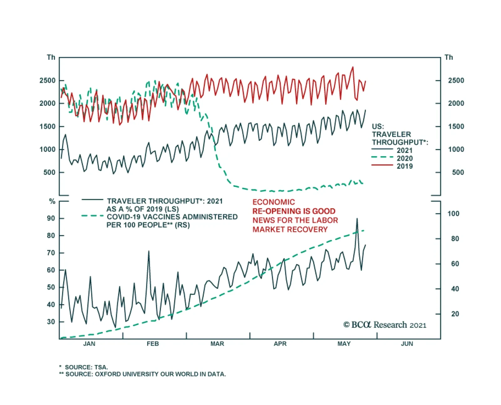
Data from the US Transportation Security Administration (TSA) suggests that US economic activity is normalizing rapidly. The number of travelers screened at TSA checkpoints in US airports continues to make fresh pandemic highs. Over the past week, that…
Highlights Domestic and foreign supply-side constraints are now exerting a significant effect on the US economy. Consumer prices may increase at a faster pace than we initially expected over the coming 3-4 months, but supply-side constraints are likely to wane later this year and thus do genuinely appear to be transitory. The idea that even a temporary period of high inflation could persist over the longer term has legitimate grounding in macro theory, and is explicitly recognized in the Fed’s inflation framework. But it would necessitate a very large increase in inflation expectations, which have yet to rise to abnormal levels. The baseline for inflation has shifted back closer to the Fed’s target, but deviations above or below target over the coming 12-18 months are likely to be driven by demand-side rather than supply-side factors. The Fed’s checklist for liftoff now entirely depends on employment, and there are compelling arguments in favor of outsized jobs growth in the second half of the year that would move forward the timing of the first rate hike. But the reality for investors is that there is tremendous uncertainty concerning the magnitude of these job gains, given the likelihood of some lasting changes to consumer behavior following the pandemic. Visibility about the employment consequences of these changes will remain very low until investors receive more information about likely urban office footprint and downtown commuter presence, the speed at which international travel will return, and to what degree any pandemic control measures remain in place in the second half of the year. For now, investors should remain cyclically overweight stocks versus bonds, short duration, and invested in other procyclical positions, with an eye to reassess the monetary policy and growth outlook in the late summer / early fall. Feature Chart I-1Investors Have Focused On The April Jobs And Inflation Data
Investors Have Focused On The April Jobs And Inflation Data
Investors Have Focused On The April Jobs And Inflation Data
Investors’ attention in May was focused squarely on two, ostensibly contradictory US data surprises: an extremely disappointing April jobs report, and a surge in consumer prices (Chart I-1). Abstracting from the typically lagging nature of consumer prices, a weak labor market is typically disinflationary / deflationary, not inflationary. But this is only to be expected in a typical environment where demand-side factors are predominantly driving the jobs market and the pricing decisions of firms, and the April data has made it clear that domestic and foreign supply-side constraints are now exerting a significant effect on the US economy, more forcefully than we initially thought. This warrants a further analysis of our prior view that supply-side effects would have a moderate effect on activity and prices this year, which we present below. A Deep Dive Into April’s Employment And Inflation Data Chart I-2 shows the difference between the April monthly gain in US jobs by industry compared with those of March. Almost all US industries saw a slower pace of jobs gains in April than March, but the slowdown was particularly acute in the professional & business services, transportation & warehousing, education & health services, construction, and manufacturing industries. By contrast, leisure & hospitality, the industry with the largest employment gap relative to pre-pandemic levels, saw a faster pace of April job gains relative to March. Chart I-2Breaking Down Disappointing April Payroll Gains
June 2021
June 2021
In our view, several facts from the April jobs report characterize the labor market as being in a transition towards a post-pandemic state, but also legitimately impacted by labor supply constraints at the low-skilled and blue-collar levels: Within professional & business services, almost all of the slowdown in monthly job gains occurred within temporary help services. Temp help services is a cyclical employment category over the longer-term, but over short periods of time it can also be negatively correlated with gains in full-time positions. April saw a large decline in the number of employed persons at work part time, suggesting that the slowdown in temp help may reflect a shift back to full-time work. Within transportation & warehousing, the slowdown in jobs was entirely attributed to the couriers and messengers subsector, which includes delivery services. In combination with the acceleration in jobs in the leisure & hospitality sector, this likely reflects a shift away from home food delivery towards in-person restaurant orders and the use of aggressive hiring tactics by restaurant owners (including advertisements of cash bonuses following 90 days of completed work, paid vacations, health insurance, and other perks). The slowdown in jobs growth in the construction & manufacturing industries is likely due to two, separate supply constraints: the negative impact of higher input costs such as lumber, semiconductors, and other raw materials, as well as the disincentivizing effects of supplementary unemployment benefits that appears to be limiting the willingness of lower-wage workers to return to work. Chart I-3April's Rise In Core CPI Was Extreme, Even After Removing Some Outliers
April's Rise In Core CPI Was Extreme, Even After Removing Some Outliers
April's Rise In Core CPI Was Extreme, Even After Removing Some Outliers
On the inflation front, Chart I-3 highlights that the April surge in core consumer prices did not just occur because of year-over-year base effects, but because of significant month-over-month increases in prices. Outsized gains in used car prices driven by the impact of the semiconductor shortage on new car production, as well as surging airline fares, did significantly contribute to April’s month-over-month gain, but the dotted line in the chart highlights that the monthly change would still have been extreme relative to history even if these components had increased instead at a 2% annual rate. Taken together, the April employment and inflation data, in conjunction with surveys of US firms as well as the trend in commodity prices, suggest that the labor market and consumer prices are being affected by four separate but related factors: An underlying demand effect, driven by extremely stimulative fiscal & monetary policy as well as economic reopening; A domestic labor shortage Coordination failures and bottlenecks impacting the production of key supply chain components and resource inputs Coordination failures and bottlenecks impacting the logistics of international trade Strong domestic aggregate demand is not likely to wane over the coming 6-12 months, which has been the basis for our view that inflation would rise to modestly above-target levels this year. Given this new evidence of their prominence and impact, it does seem likely that the remaining three supply-side factors will persist for a few more months, suggesting that core inflation may remain quite elevated over the near term. But several points underscore why it remains difficult to accept a view that supply-side factors will remain an important driver of employment and consumer price trends on a 1-year time horizon. Chart I-4Home Schooling Is Impacting The Labor Market
June 2021
June 2021
First, domestic labor shortages are occurring in the context of a gap of 8.2 million jobs relative to pre-pandemic levels, underscoring that substantial barriers to returning to work exist. The three most cited barriers are an unwillingness to return to employment for health reasons, an unwillingness to return to work because of supplementary unemployment insurance benefits that are in excess of regular income, and an inability to return to work due to childcare requirements. For example, Chart I-4 highlights that the labor force participation rate has declined the most for women with young children, whose children in many cases are being schooled online rather that in person. But all three of these factors are clearly linked to the pandemic, and are likely to be greatly reduced (or eliminated) in the fall once schools have reopened and income support has ended. Federal supplementary UI benefits are set to expire by labor day, and several US states have already opted out of the program – with benefits set to end in June or July.1 Second, global producers of important commodity inputs (such as lumber) significantly cut production last year under the expectation that the pandemic would greatly reduce spending, only to be whipsawed by a surge in demand stemming from a combination of working from home effects and a massive policy response. Chart I-5 highlights that US industrial production of wood products fell to -10% on a year-over-year basis last April, but that it has subsequently rebounded to a new high. Unlike other supply chain inputs, global semiconductor sales did not decline last April (in the face of enormous PC, tablet, and server/data center demand), but Chart I-6 highlights that DRAM prices, lumber prices, and prices of raw industrial goods may be peaking or have already peaked. Chart I-5Lumber Prices Are Soaring, In Part, Because Supply Was Cut Last Year
Lumber Prices Are Soaring, In Part, Because Supply Was Cut Last Year
Lumber Prices Are Soaring, In Part, Because Supply Was Cut Last Year
Chart I-6Costs of Key Inputs May Be Peaking (Or Have Peaked)
Costs of Key Inputs May Be Peaking (Or Have Peaked)
Costs of Key Inputs May Be Peaking (Or Have Peaked)
Chart I-7Logistical Issues, Which Will Be Resolved, Are Driving Shipping Costs
Logistical Issues, Which Will Be Resolved, Are Driving Shipping Costs
Logistical Issues, Which Will Be Resolved, Are Driving Shipping Costs
Third, while some market participants have attributed the enormous rise in global shipping costs entirely to the underlying demand effect that we noted above, Chart I-7 highlights that this is clearly not the case. The chart shows that the surge in loaded inbound container trade to the Los Angeles and Long Beach ports, to its strongest level since the inception of the data in the mid 1990s, could potentially explain a 75-100% year-over-year rise in shipping costs – less than half of the 250% surge that has occurred over the past 12 months. This strongly points to logistical issues such as the incorrect positioning of cargo containers amid pandemic-related port congestion (and other disruptions such as the temporary grounding of the Ever Given in the Suez canal) as the dominant driver of global shipping costs, which have likely pushed up US non-oil import prices by more than what would normally be implied by the decline in the US dollar (Chart I-8). Global shipping costs have yet to peak, but we expect that these logistical problems will likely be resolved sometime in Q3, or potentially over the summer. This view is underpinned by the fact that the number of global container ships arriving on time rose in March, the first month-over-month increase since June of last year.2 Chart I-8Rising Transport Costs Have Pushed Up US Import Prices
Rising Transport Costs Have Pushed Up US Import Prices
Rising Transport Costs Have Pushed Up US Import Prices
For investors, the key conclusion of this review is that while consumer prices may increase at a faster pace than we initially expected over the coming 3-4 months, supply-side factors are clearly driving outsized gains, and have likely or definite end points before the end of the year. As such, despite the surprising magnitude of these supply-side factors, they do genuinely appear to be transitory. The “Transitory” Debate Most investors would agree that 3-4 months of outsized consumer price increases would not be, in and of themselves, economically significant or investment relevant. But the question of whether even a temporary period of high inflation could persist over a 12-month or multi-year time horizon has become prominent in the marketplace, with some investors believing that it has high odds of fueling an already-established, demand-side narrative supporting higher prices in a way that becomes self-reinforcing among consumers and firms. Indeed, this view has a legitimate grounding in macro theory, and is explicitly recognized in the Fed’s inflation framework – which is called the expectations-augmented or Modern-Day Phillips Curve (“MDPC”). In anticipation of the coming debate about inflation and its causes, we thoroughly reviewed the MDPC in our January report.3 One crucial takeaway from the MDPC framework is that economic activity relative to its potential determines the degree to which inflation deviates from expectations of inflation, not the Fed’s inflation target. If, for example, inflation expectations are meaningfully below target, then the Fed would need to aim for an unemployment rate below its natural rate for some period of time in an attempt to re-anchor expectations closer to its target rate (based on the view that inflation expectations adapt to the actual inflation experience). This is essentially what occurred in the latter half of the last economic expansion, and is what motivated the Fed’s shift to its average inflation targeting regime. The Modern-Day Phillips Curve is “modern” because of the experience of inflation in the late 1960s and 1970s, where ever-rising expectations for inflation (alongside extremely easy monetary policy) became self-reinforcing and caused core PCE inflation to rise to high single-digit territory in the second half of the decade. Thus, the notion that elevated consumer prices over the short-term could increase actual inflation over the longer term via higher expectations – meaning that it would not be transitory – is plausible. Chart I-9The Fed's New Index Of Common Inflation Expectations (CIE)
The Fed's New Index Of Common Inflation Expectations (CIE)
The Fed's New Index Of Common Inflation Expectations (CIE)
Is it likely? In our view, while the odds have increased somewhat over the past month, the answer is no. Chart I-9 presents the Fed’s quarterly index of common inflation expectations (CIE), alongside a model designed to track movements in the index on a monthly frequency. While the Fed’s index includes over 21 inflation expectation indicators, our condensed model uses just six: the 10-year annualized rate of change in headline inflation, the 10-year annualized rate of change in the headline PCE deflator, 5-year/5-year forward and 10-year/10-year forward TIPS breakeven inflation rates, the 3-month moving average of long-term surveyed consumer expectations for inflation, and a proprietary measure of inflation expectations based on an adaptive expectations framework. Chart I-10 highlights that among these six series (shown standardized since mid 2004), three of them have risen quite significantly over the past year: long-dated TIPS breakeven inflation rates (5-5 and 10-10), and long-term consumer expectations for inflation. In our view, the latter series from the University of Michigan is one of the most important for investors to monitor over the coming year, as it is one of the few available measures of “main-street” inflation expectations with a long history. Chart I-10Important Drivers Of The CIE Index Have Risen, But From A Low Base
Important Drivers Of The CIE Index Have Risen, But From A Low Base
Important Drivers Of The CIE Index Have Risen, But From A Low Base
Chart I-11A Deeply Negative Output Gap Last Cycle Made Inflation Expectations Vulnerable To Shocks
A Deeply Negative Output Gap Last Cycle Made Inflation Expectations Vulnerable To Shocks
A Deeply Negative Output Gap Last Cycle Made Inflation Expectations Vulnerable To Shocks
But while the series in the top panel of Chart I-10 have risen sharply, they are rising from an extremely low base and are currently only fractionally above their average since 2004. As noted in our January report, inflation expectations fell significantly in 2014 first because they were highly vulnerable to shocks following a long period of a deeply negative output gap (Chart I-11), and second because they were catalyzed by a substantial US dollar / oil price shock that occurred in that year. We noted above that the odds of extreme near-term price changes ultimately becoming non-transitory have risen somewhat, and Chart I-12 highlights why. The chart presents the annual change in long-term consumer expectations of inflation alongside the annual change in 2-year government bond yields, and notes that the past three cases of a similar-sized spike in expectations were all ultimately met with either a significant rise in short-term interest rates or a major deflationary shock – neither of which we expect to occur over the coming year. Chart I-12Other Consumer Price Expectation Spikes Have Been Met By Rising Rates Or A Deflationary Shock
Other Consumer Price Expectation Spikes Have Been Met By Rising Rates Or A Deflationary Shock
Other Consumer Price Expectation Spikes Have Been Met By Rising Rates Or A Deflationary Shock
However, the fact that the rise in expectations clearly has a mean-reversion component to it, and that the supply-side factors driving month-over-month price increases are temporary in nature, argues against the idea that expectations will rise above the average that prevailed from 2002 – 2014. This suggests that while the baseline for inflation has moved back closer to the Fed’s target, deviations above or below target are likely to be driven by demand-side rather than supply-side factors. The Fed’s Checklist: Focus On Employment Table I-1The Fed’s Checklist For Liftoff
June 2021
June 2021
From an investment perspective, the outlook for inflation is important mostly because of its implications for Fed policy, and thus interest rates and equity valuation multiples. My colleague Ryan Swift, BCA’s US Bond Strategist, has presented the Fed’s checklist for liftoff in Table I-1. The Fed has been explicit that they will not raise interest rates until all three boxes are checked, regardless of what is occurring to inflation expectations or actual inflation. The first box in the list is essentially checked, as tomorrow’s April Personal Income and Outlays report will very likely confirm that the core PCE deflator rose in excess of 2% (the headline PCE deflator was already in excess of this in March). And the third criterion is essentially a derivative of the other two, barring the emergence of a significant deflationary shock at the time that the Fed would otherwise begin to raise rates. This means that investors should be entirely focused on labor market developments, and whether they are consistent with the Fed’s assessment of maximum employment. Table I-2 highlights the average monthly nonfarm payroll growth that will be required for the unemployment rate to reach 3.5-4.5%, the range of the Fed’s NAIRU estimates. The table underscores that large gains will be required for the Fed’s maximum employment criteria to be met by the end of this year or year-end 2022, on the order of 410-830k per month. Table I-2Calculating The Distance To Maximum Employment
June 2021
June 2021
But the nature of the pandemic and the factors that drove what is still an 8.2 million jobs gap underscore the extreme difficulty in forecasting what monthly job gains are likely to occur on average over the coming 12-18 months. From March to August of last year, monthly changes in nonfarm payrolls exceeded +/-1 million per month, with 20.7 million jobs lost in the month of April 2020 alone. Payroll gains averaged 3.8 million per month in the two months that followed, and if that pace were to be repeated this fall as schools reopen and supplementary unemployment benefits draw to a close in all states it would close 93% of the outstanding jobs gap. This implies that monthly job growth will follow a bimodal distribution over the coming year, with large gains in Q3/Q4 followed by a much more normal pace of jobs growth in Q1/Q2 2022. In our view, the outlook for Fed policy depends significantly on the magnitude of those outsized gains in employment this fall, and there are three main arguments favoring a larger pace of monthly job growth during this period. First, Table I-3 highlights that the jobs gap is most prominent in the leisure & hospitality, government, education & health services, and professional & business services industries, and several observations suggest that Q3/Q4 job gains in these sectors may be sizeable: Table I-3Breaking Down The Pandemic Employment Gap By Industry
June 2021
June 2021
70% of the government employment gap shown in Table I-3 can be attributed to education, as government employment also includes education employment at the state and local government level. Many of these jobs, along with those in the education & health services industry, are likely to recover in the fall as schools reopen across the country. As noted in our discussion of the April jobs data, the professional & business services industry includes the “administrative & support services” sector, which accounts for 85% of the overall job gap for the industry. These jobs have likely been impacted heavily by reduced office presence as well as business travel, and may recover further in the fall as many employees shift partially or fully away from working from home. Chart I-13Leisure & Hospitality Employment Is Closely Tracking Hotel Occupancy
Leisure & Hospitality Employment Is Closely Tracking Hotel Occupancy
Leisure & Hospitality Employment Is Closely Tracking Hotel Occupancy
Chart I-13 highlights that the year-over-year growth rates of leisure & hospitality employment and the US hotel occupancy rate are tracking each other quite closely, and that the latter is in a solid uptrend.4 While international travel is likely to remain muted this summer, the rebound in hotel occupancy suggests that Americans are choosing to travel domestically this year and that further gains in occupancy may occur over the coming months. Chart I-14 highlights the second argument in favor of a larger pace of monthly job growth in the second half of the year. The chart shows the clear relationship between reopening and the employment gap, with states that have fully reopened having substantially smaller gaps than states that have not. It is true that some states that have fully reopened are still experiencing a sizeable gap, but this is at least in part due to leisure & hospitality employment that is dependent on the travel patterns of consumers. For example, Nevada still has a 10% employment gap despite having fully reopened, clearly reflecting the impact of reduced tourism to Las Vegas. Thus, as all states move towards being fully reopened later this year, including large states such as New York and California, Chart I-14 suggests that the US jobs gap is likely to narrow significantly. Chart I-14US States That Have Reopened Have A Smaller Employment Gap
June 2021
June 2021
Chart I-15Real Output Per Worker Is Not Likely To Rise Further
Real Output Per Worker Is Not Likely To Rise Further
Real Output Per Worker Is Not Likely To Rise Further
Finally, Chart I-15 highlights that the 2020 recession is the only one in which real output per person rose sharply during the recession. It is true that productivity tends to rise over time and that it usually increases in the early phase of an economic recovery, but the rise in real output per worker last year clearly reflects the massive decline in employment and services spending that resulted from pandemic-related control measures and lockdowns. Our sense is that this sharp rise in real output per worker is not likely to be sustained following full reopening and the elimination of barriers to employment, and if real output per worker were to even modestly converge to its prior trend (the dotted line in Chart I-15) it would more than fully close the jobs gap shown in Table I-3 by the end of the year based on consensus growth forecasts for this year. Investment Conclusions Despite compelling arguments for outsized jobs growth in the second half of the year, the bottom line for investors is that there is tremendous uncertainty concerning its magnitude. It seems likely that there will be some lasting changes to consumer behavior following the pandemic, and visibility about the employment consequences of these changes will remain very low until investors receive more information about the likely urban office footprint and downtown commuter presence, the speed at which international travel will return, and the degree to which any pandemic control measures remain in place in the second half of the year. Given the Fed’s criteria for liftoff, developments that imply a pace of jobs recovery that is in line with or slower than the Fed’s unemployment rate projections will ensure that the monetary policy regime will remain supportive of risky asset prices over the coming year. If the employment gap closes rapidly in Q3/Q4, then investor expectations for the timing of the first rate hike will move sharply closer, which could act as a negative inflection point for stock prices. This is now more probable than it was a month ago, as Chart I-16 highlights that the OIS curve has shifted towards expectations of an initial rate hike at the end of next year or early 2023, from mid 2022 previously. Chart I-16Market Rate Hike Expectations Have Shifted Back To Late 2022 / Early 2023
Market Rate Hike Expectations Have Shifted Back To Late 2022 / Early 2023
Market Rate Hike Expectations Have Shifted Back To Late 2022 / Early 2023
Still, abstracting from knee-jerk market reactions, it is the pace of hikes and investor expectations for the terminal Fed funds rate that are the more important fundamental drivers of 10-year Treasury yields, and investors would need to see a very large revision to the latter in order for yields to rise to a point that would restrict economic activity or threaten equity market multiples. Such a revision is highly unlikely over the summer unless incoming evidence strongly suggests that the employment gap will be closed by the end of the year. As highlighted above, this may indeed occur later in the year, but probably not over the coming 3 months. For now, investors should remain cyclically overweight stocks versus bonds, short duration, and invested in other procyclical positions, with an eye to reassess the monetary policy and growth outlook in the late summer / early fall. Jonathan LaBerge, CFA Vice President The Bank Credit Analyst May 27, 2021 Next Report: June 24, 2021 II. Global House Prices: A New Threat For Policymakers House prices are rising rapidly across the developed markets, in response to the extraordinary monetary and fiscal policy stimulus implemented to fight the pandemic. Evidence points to the house price surge being driven by monetary policy that has left real interest rates far below equilibrium levels. Supply factors are a secondary cause of the house price boom. Financial stability risks stemming from rising house prices are less acute than the pre-2008 experience, as overall household leverage has grown more slowly during the pandemic and global banks are better capitalized. Rapidly rising house prices are forcing some central banks to turn less accommodative earlier than expected. The recent hawkish turns by the Bank of Canada and Reserve Bank of New Zealand may be canaries in the coal mine for other central banks – perhaps even the Fed – if house prices and household leverage start rising together. The COVID-19 pandemic led to the sharpest economic recession since World War II, alongside an enormous rise in unemployment. Consensus expectations call for the output gap to be closed (or mostly closed) in most advanced economies by the end of this year, but it remains an open question how quickly these economies will be able to return to full employment amid potentially permanent shifts in demand for office space and goods sold at physical, “brick and mortar” retail locations. Despite this sizeable and swift economic shock, house price appreciation accelerated last year in the developed world. Chart II-1 highlights that US house prices rose at an 18% annualized pace in the second half of 2020, whereas they accelerated at a high-single digit pace in developed markets ex-US (on a GDP-weighted basis). This, in conjunction with a sharp rise in the household sector credit-to-GDP ratio (Chart II-2), has unnerved some investors while raising questions about the implications for monetary policy. Chart II-1House Prices Are Surging Around The World
House Prices Are Surging Around The World
House Prices Are Surging Around The World
Chart II-2Rising Fears About Deteriorating Household Balance Sheets
Rising Fears About Deteriorating Household Balance Sheets
Rising Fears About Deteriorating Household Balance Sheets
Before we discuss the investment implications of the global housing boom, however, we must first accurately determine the reasons why it is happening. The Work-From-Home Effect: Less Than Meets The Eye When analyzing the surprising behavior of the housing market last year, the working-from-home effect brought upon by the pandemic emerges as an obvious factor potentially explaining house price gains. Last year, following recommended or mandatory stay-at-home orders from governments, most office-based businesses rapidly shifted to work-from-home arrangements as an emergency response. However, in the month or two following the beginning of stay-at-home orders, several national US surveys found many office workers preferred the flexibility afforded by work-from-home arrangements. Many employers, correspondingly, found that the productivity of their employees did not suffer while working from home, or that it even improved. Several prominent corporations in the US have subsequently made some work-from-home options permanent, or even allowed employees to work from offices in a different city than they did prior to the pandemic. Newfound work-from-home options have undoubtedly created new demand for housing, and thus explained the surge in house prices seen over the past year in the minds of some investors. However, in our view, evidence from the US, the UK, and France suggests that the work-from-home effect better explains differences in price gains across housing types and within large metropolitan areas, rather than aggregate or national-level changes in house prices. Chart II-3 provides some quantification of the impact of work-from-home policies by plotting US resident migration patterns by city. This data has been compiled by CBRE, and the impact of COVID is shown as the change in net move-ins from 2019 to 2020 per 1000 people. This helps control for the underlying migration pattern that existed in US cities prior to the pandemic. Chart II-3Work From Home Policies Have Impacted Migration Trends…
June 2021
June 2021
The chart highlights that the negative migration impact from COVID has been mostly concentrated in New York City and the three most populous cities on the West Coast (by metro area): Los Angeles, San Francisco, and Seattle. And yet, Chart II-4 highlights that house price inflation in these four cities has accelerated to a double-digit pace, only modestly below the national average. Chart II-4...But Cities With Outward Migration Still Have Very Strong House Price Gains
...But Cities With Outward Migration Still Have Very Strong House Price Gains
...But Cities With Outward Migration Still Have Very Strong House Price Gains
The house price indexes shown in Chart II-4 represent aggregate, metro area trends, and clearly some regions within these metro areas have experienced house price deceleration or outright deflation versus gains in areas outside the urban core. But Chart II-5 highlights that house prices have declined in Manhattan basically in line with the change in net move-ins as a share of the population, underscoring that double-digit metro area-wide house price gains appear to be vastly disproportionate to changes in net migration. Similarly, Chart II-6 highlights that rents decelerated in the US over the past year but remained in positive territory and grew at a 3.5% annualized rate from February to April. Chart II-5In Manhattan, House Prices Have Tracked Net Migration
June 2021
June 2021
Chart II-6Rent Costs Have Decelerated, But Have Not Contracted
Rent Costs Have Decelerated, But Have Not Contracted
Rent Costs Have Decelerated, But Have Not Contracted
Evidence from Paris and London also suggests that a work-from-home effect is insufficient to explain broad house price gains. Panel 1 of Chart II-7 highlights that house prices in France have accelerated significantly, but that apartment prices have decelerated only fractionally in lockstep. Panel 2 shows that the acceleration in house prices does reflect a work-from-home effect, as prices have risen faster in inner Parisian suburbs. Panel 3, however, highlights that Parisian apartment prices, the dominant property type in the urban core, have decelerated modestly. Chart II-8 highlights that house price gains have not even decelerated in greater London; they have been merely been modestly outstripped by gains in Outer South East (outside of the Outer Metropolitan Area). Chart II-7In France, Parisian Apartment Prices Are Simply Lagging, Not Falling
In France, Parisian Apartment Prices Are Simply Lagging, Not Falling
In France, Parisian Apartment Prices Are Simply Lagging, Not Falling
Chart II-8In The UK, Greater London Property Prices Are Accelerating
In The UK, Greater London Property Prices Are Accelerating
In The UK, Greater London Property Prices Are Accelerating
The Policy Effect: The Fundamental Driver Of The Housing Market Despite the broader location flexibility that work-from-home policies now provide to potential homeowners, it seems inconceivable that the housing market would have responded in the manner that it has over the past year given the size of the economic shock brought on by the pandemic without significant support from policy. Above-the-line fiscal measures to the pandemic have totaled in the double-digits in advanced economies (Chart II-9), and monetary policy has contributed to easier financial conditions via rate cuts, asset purchases, and sizeable programs to support financial market liquidity. Chart II-9There Has Been A Massive Fiscal Policy Response To The Crisis
June 2021
June 2021
In fact, Charts II-10-II-13 present compelling evidence that fiscal and monetary policy have been the core drivers of significant house price gains over the past year. Charts II-10 and II-11 plot the above-the-line fiscal response of advanced economies against the year-over-year growth rate in house prices as well as its acceleration (the change in the year-over-year growth rate). The charts show a clearly positive relationship, with a stronger link between the pandemic fiscal response and the acceleration in house prices. Chart II-10Differences In Last Year’s Fiscal Response…
June 2021
June 2021
Chart II-11…Help Explain Differences In House Price Gains
June 2021
June 2021
Chart II-12Pre-Pandemic Differences In The Monetary Policy Stance…
June 2021
June 2021
Chart II-13…Do An Even Better Job Of Explaining 2020 House Price Gains
June 2021
June 2021
Charts II-12 and II-13 highlight the even stronger link between house prices and the pre-pandemic monetary policy stance in advanced economies, defined as the difference between each country’s 2-year government bond yield and its Taylor Rule-implied policy interest rate as of Q4 2019. We construct each country’s Taylor Rule using the original specification, with core consumer price inflation, a 2% inflation target, and real potential GDP growth as the definition of the real equilibrium interest rate. The charts make it clear that easy monetary policy strongly explains house price gains in 2020, particularly the year-over-year percent change rather than its acceleration. This makes sense, given that monetary policy was already quite easy in many countries at the onset of the pandemic – meaning that changes were less pronounced than they would have been had interest rates been higher. The explanation that emerges from Charts II-10-II-13 is that historic fiscal easing, combined with an easy starting point for monetary policy – that became even easier last year – enabled demand from work-from-home policies to manifest during an extremely severe recession. We agree that work-from-home policies have shifted the geographic preferences of some home buyers and likely provided a new source of net demand from renters in urban cores purchasing homes in outlying areas. But we strongly doubt that the net effect of work-from-home policies in the midst of an extreme shock to economic activity would have caused the rise in house prices that we have observed, certainly not to this level, without major support from policy. This underscores that policy, and not the work-from-home effect, has and will likely remain the core driver of the global housing market. The Supply Effect: Mostly A Red Herring Chart II-14Countries Fall Into Two Groups In Terms Of The Relative Trend In Real Residential Investment
Countries Fall Into Two Groups In Terms Of The Relative Trend In Real Residential Investment
Countries Fall Into Two Groups In Terms Of The Relative Trend In Real Residential Investment
One perennial question that emerges when analyzing the housing market, particularly in markets with outsized house price gains, is the impact of constrained supply. It is frequently argued that constrained supply is squeezing prices higher in many markets, and that the appropriate policy solution to extreme house price gains is to enable widespread housing construction – not to raise interest rates. We do not rule out the potential impact of constrained supply in certain cities or regional housing markets, and we have highlighted in previous research that a positive relationship does exist between population density in urban regions and median house price-to-income ratios.5 But as a broad explanation for supercharged house price gains, the supply argument appears to fall flat. Chart II-14 presents the most standardized measure of cross-country housing supply available for several advanced economies, the trend in real residential investment relative to real GDP over time. These series are all rebased to 100 as of 1997, prior to the 2002-2007 US housing market boom. The chart makes it clear that advanced economies generally fall into two groups based on this metric: those that have seen declines in real residential investment relative to GDP, especially after the global financial crisis (panel 1), and those that have experienced either an uptrend in housing construction relative to output or have seen a flat trend (panel 2). If scarce housing supply was the core driver of outsized house price gains, then we would expect to see stronger gains in the countries shown in panel 1 and smaller gains in the countries shown in panel 2. In fact, mostly the opposite is true: Charts II-15 and II-16 highlight that the relationship between the level of these indexes today relative to their 1997 or 2005 levels is positively related to the magnitude of house price gains last year, suggesting that housing market supply has generally been responding to demand over the past decade. The US and possibly New Zealand stand as possible exceptions to the trend, suggesting that relatively scarce supply may be boosting prices even further in these markets beyond what fiscal and monetary policy would suggest. Chart II-15Countries That Have Seen A Stronger Pace Of Residential Investment…
June 2021
June 2021
Chart II-16…Have Experienced Stronger House Price Gains
June 2021
June 2021
Chart II-17Is This Not Enough Supply, Or Too Much Demand?
June 2021
June 2021
As a final point about the inclination of investors to gravitate towards supply-side arguments related to the housing market, Chart II-17 presents a simple thought experiment. The chart shows a simple housing supply-demand curve diagram, in a scenario where the demand curve for housing has shifted out more than the supply curve has (thus raising house prices). Is this a scenario in which supply is too tight? Or is it a case in which demand is too strong? In our view, the tight supply answer is reasonable in circumstances where the increase in demand is normal or otherwise sustainable. But Charts II-10-II-13 clearly showed that housing demand is being boosted by easy policy, which in the case of some countries has occurred for years: interest rates have remained well below levels that macroeconomic theory would traditionally consider to be in equilibrium, and this has occurred alongside significant household sector leveraging (Chart II-18). As such, in our view, investors should be more inclined to view the global housing market as generally being driven by demand-side rather than supply-side factors. This Is Not 2007/08 … Yet We highlighted in Chart II-2 above that the household sector debt-to-GDP ratio increased sharply last year, which has raised some questions about debt sustainability among investors. For the most part, the rise in this ratio actually reflects denominator effects (namely a sharp contraction in nominal GDP) rather than a huge surge in household debt. Chart II-19 shows BIS data for the annual growth in total household debt in developed economies was roughly stable last year, at least until Q3 (the most recent datapoint available from the BIS). Chart II-18Low Interest Rates Have Fueled Household Leveraging
Low Interest Rtaes Have Fueled Household Leveraging
Low Interest Rtaes Have Fueled Household Leveraging
Chart II-19Total Credit Growth Has Been Stable, But Mortgage Credit Growth Is Accelerating
Total Credit Growth Has Been Stable, But Mortgage Credit Growth Is Accelerating
Total Credit Growth Has Been Stable, But Mortgage Credit Growth Is Accelerating
Chart II-20US Mortgage Growth Is Picking Up, As Repayments Slow Consumer Credit Growth
US Mortgage Growth Is Picking Up, As Repayments Slow Consumer Credit Growth
US Mortgage Growth Is Picking Up, As Repayments Slow Consumer Credit Growth
But Chart II-19 shows the recent trend in total household debt, which masks diverging mortgage and non-mortgage debt trends. In the US, euro area, Canada, and Sweden, household mortgage debt has accelerated to varying degrees, underscoring that households have likely paid down non-mortgage debt with some of the savings that they have accumulated from a significant reduction in spending on services. Chart II-20 shows this effect directly in the case of the US; mortgage debt growth accelerated by roughly 1.5 percentage points in the second half of the year, whereas consumer credit growth (made up of student loans, auto loans, credit cards, and other revolving credit) decelerated significantly. This aligns with data showing that US households have used some of their savings windfall to pay down their credit card balances. This changing mix within household debt - less higher-interest-rate consumer credit, more lower-interest-rate collateralized mortgage debt – could, on the margin, help mitigate financial stability risks from the housing boom by moderating overall debt service burdens. The starting point for the latter matters, though, in accurately assessing the risks from rising house prices and increased mortgage debt, particularly in countries where household debt levels are already high. According to data from the BIS, the US already has one of the lowest household debt service ratios (7.6%) among the developed economies (Chart II-21).6 This compares favorably to the double-digit debt service ratios in the “higher-risk” countries like Canada (12.6%), Sweden (12.1%) and Norway (16.2%). On top of that, US commercial banks have become far more prudent with mortgage loan underwriting standards since the 2008 financial crisis. The New York Fed’s Household Debt and Credit report shows that an increasing majority of mortgage lending made by US banks since the 2008 crisis has been to those with very high FICO credit scores (Chart II-22). This is in sharp contrast to the steady lending to “subprime” borrowers with poor credit scores that preceded the 2008 financial crisis. The median FICO score for new mortgage originations as of Q1 2021 was 788, compared to 707 in Q4 2006 at the peak of the mid-2000s US housing boom. Chart II-21Diverging Trends In Global Household Debt Servicing Costs
Diverging Trends In Global Household Debt Servicing Costs
Diverging Trends In Global Household Debt Servicing Costs
Chart II-22US Banks Have Become More Prudent With Mortgage Lending
US Banks Have Become More Prudent With Mortgage Lending
US Banks Have Become More Prudent With Mortgage Lending
US bank balance sheets are also now less directly exposed to a fall in housing values. Residential loans now represent only 10% of the assets on US bank balance sheets, compared to 20% at the peak of the last housing bubble (Chart II-23). This puts the US in the “lower-risk” group of countries in Europe, the UK and Japan where mortgages are less than 20% of bank balance sheets. This compares favorably to the “higher risk” group of countries where residential loans are a far larger share of bank assets (Chart II-24), like Canada (32%), New Zealand (49%), Sweden (45%) and Australia (40%). Chart II-23Banks Have Limited Direct Exposure To Housing Here
Banks Have Limited Direct Exposure To Housing Here
Banks Have Limited Direct Exposure To Housing Here
Chart II-24Banks Are Far More Exposed To Housing Here
Banks Are Far More Exposed To Housing Here
Banks Are Far More Exposed To Housing Here
Like nature, however, the financial ecosystem abhors a vacuum. “Non-bank” mortgage lenders have filled the void from traditional US banks reducing their lending to lower-quality borrowers, and they now represent around two-thirds of all US mortgage origination, a big leap from the 20% origination share in 2007. Non-bank lenders have also taken on growing shares of new mortgage origination in other countries like the UK, Canada and Australia. Chart II-25Global Banks Can Withstand A Housing Shock
June 2021
June 2021
Non-bank lenders do not take deposits and typically fund themselves via shorter-term borrowings, which raises the potential for future instability if credit markets seize up. These lenders also, on average, service mortgages with a higher probability of default, so they are exposed to greater credit losses when house prices decline. However, the risk of a full-blown 2008-style commercial banking crisis, with individual depositors’ funds at risk from a bank failure, are reduced with a greater share of riskier mortgage lending conducted by non-bank entities. This is especially true with global commercial banks far better capitalized today, with double-digit Tier 1 capital ratios (Chart II-25), thanks to regulatory changes made after the Global Financial Crisis. Net-net, we conclude that the overall financial stability implications of the current surge in house prices in the developed economies are relatively modest on average. The acceleration in mortgage growth has occurred alongside reductions in non-mortgage growth, at a time when banks are better able to withstand a shock from any sustained future downturn in house prices. However, if house prices continue to accelerate and new homebuyers are forced to take on ever increasing amounts of mortgage debt, financial stability issues could intensify in some countries. Services spending will recover in a vaccinated post-COVID world, as economies reopen and consumer confidence improves, which will likely end the trend of falling non-residential consumer debt offsetting rising mortgage debt in countries like the US and Canada. Overall levels of household debt could begin to rise again relative to incomes, building up future financial stability risks when central banks begin to normalize pandemic-related monetary policies – a process that has already started in some countries because of the housing boom. The Monetary Policy Implications Of Surging House Prices Rapidly appreciating house prices are becoming an area of concern for policymakers in countries like Canada and New Zealand, where the affordability of housing is becoming a political, as well as an economic, issue. In the case of New Zealand, the government has actually altered the remit of the Reserve Bank of New Zealand (RBNZ) to more explicitly factor in the impact of monetary policy on housing costs. The Bank of Canada announced in April that it would taper its pace of government debt purchases and signaled that its decision was based, at least in small part, on signs of speculative behavior in Canada’s housing market. Macroprudential measures like limiting loan-to-value ratios of new mortgage loans are a policy option that governments in those countries have already implemented to try and cool off housing demand. Yet while such measures can help alleviate demand-supply mismatches in certain cities and regions, the efficacy of such measures in sustainably slowing the ascent of house prices on a national scale is unclear. In the April 2021 IMF Global Financial Stability Report, researchers estimated that, for a broad group of countries, the implementation of a new macro-prudential measure designed to cool loan demand reduced national household debt/GDP ratios by a mere one percentage point, on average, over a period encompassing four years.7 If macroprudential measures are that ineffective in sustainably reducing demand for mortgage loans, then the burden of slowing house price appreciation will have to fall on the more blunt instruments of monetary policy. Importantly, surging house price inflation is not likely to give a boost to realized inflation measures – an important issue given the current backdrop of rapidly rising realized inflation rates in many countries. Housing costs do represent a significant portion of consumer price indices in many developed countries, ranging from 19% in New Zealand to 33% in the US (Chart II-26), with the euro area being the outlier with housing having a mere 2% weighting in the headline inflation index. Chart II-26A Limited Impact On Actual Inflation From Housing
June 2021
June 2021
Yet those so-called “housing” categories overwhelmingly measure only housing rental costs and not actual house prices. This is an important distinction because rents – which are often imputed measures like in the US and not even actual rental costs - are rising at a far slower pace than actual house prices in most countries, so the housing contribution to realized inflation is relatively modest. So the good news is that booming house prices will not worsen the acceleration of realized global inflation that has concerned investors and policymakers in 2021. Yet that does not mean that central bankers will not be forced to tighten policy to cool off red-hot housing demand that is clearly being fueled by persistently negative real interest rates. In Chart II-27 and Chart II-28, we show both nominal and real policy interest rates for the “lower risk” and “higher risk” country groupings that we described earlier. The real policy rates are nominal policy rates versus realized headline CPI inflation. The dotted lines in the charts represent the future path of rates discounted by markets. Specifically, the projection for nominal rates is taken from overnight index swap (OIS) forward curves, while the projection for real rates is calculated by subtracting the discounted path of inflation expectations extracted from CPI swap forwards. Chart II-27Markets Discounting Negative Real Rates For The Next Decade
Markets Discounting Negative Real Rates For The Next Decade
Markets Discounting Negative Real Rates For The Next Decade
Chart II-28Negative Real Rates Are Unsustainable During A Housing Bubble
Negative Real Rates Are Unsustainable During A Housing Bubble
Negative Real Rates Are Unsustainable During A Housing Bubble
There are two key takeaways from these charts: Real policy interest rates are at or very close to the most deeply negative levels seen since the 2008 financial crisis. Markets are discounting that real rates will be at or below 0% for most of the next decade. Admittedly, there is room for debate over what the equilibrium level of real interest rates (a.k.a. “r-star”) should be in the coming years. However, we deem it a major stretch to believe that real rates need to be persistently low or negative for the next ten years to support even trend growth across the developed economies. In our view, the current boom in housing demand and mortgage borrowing provides clear evidence that negative real rates are below equilibrium and, thus, are stimulating credit demand. Thus, the only way for a central bank to cool off housing demand will be to raise both nominal and, more importantly, real interest rates. Canada and New Zealand will be the “canaries in the coal mine” among developed market central banks for such a move. According to the latest Bank of Canada Financial Stability Review, nearly 22% of Canadian mortgages are highly levered, with a loan-to-value ratio greater than 450%, a greater share of such mortgages than during the 2016/17 housing boom (Chart II-29). Canadian house prices have risen to such an extent that home prices in major cities like Toronto, Vancouver and Montreal are among the most expensive in North America.8 Stunningly, a recent Bloomberg Nanos opinion poll revealed that nearly 50% of Canadians would support Bank of Canada rate hikes to cool off the red-hot housing market (Chart II-30). The central bank will be unable to resist the pressure to use monetary policy to slam on the brakes of the housing market – investors should expect more tapering and, eventually, rate hikes from the Bank of Canada over at least the next couple of years. Chart II-29Canadians Are Leveraging Up To Buy Expensive Homes
Canadians Are Leveraging Up To Buy Expensive Homes
Canadians Are Leveraging Up To Buy Expensive Homes
Chart II-3050% Of Canadians Want A Rate Hike To Cool Housing
June 2021
June 2021
In New Zealand, worsening housing affordability has reached a point where a 20% down payment on the median national house price is equal to 223% of median disposable income (Chart II-31). This is forcing more first-time home buyers to take on levels of mortgage debt that the RBNZ deems highly risky (top panel). Like the Bank of Canada, the RBNZ will prove to be one of the most hawkish central banks in the developed world over the next couple of years as the central bank follows their newly-revised remit to try and cool off housing demand in New Zealand. Who is next? Housing values, measured by the ratio of median national house prices to median national household incomes, are rising in the US and UK but are still below the peaks of the mid-2000s housing bubble (Chart II-32). Meanwhile, housing is becoming more expensive across the euro area, but not in a consistent manner, with valuations in Germany and Spain having increased far more than in France or Italy. Housing valuations have actually improved in Australia over the past couple of years on a price-to-income basis. The most likely candidates for a housing-related hawkish turn are in Scandinavia, with housing valuations in Sweden and Norway closing in on Canada/New Zealand levels. Chart II-31New Zealand Housing Is Wildly Unaffordable
New Zealand Housing Is Wildly Unaffordable
New Zealand Housing Is Wildly Unaffordable
Chart II-32Global House Price/Income Ratios Are Trending Higher
Global House Price/Income Ratios Are Trending Higher
Global House Price/Income Ratios Are Trending Higher
Investment Conclusions The current acceleration in global house prices is an inevitable outcome of the extraordinary monetary and fiscal easing implemented during the pandemic. Higher realized inflation is pushing real rates deeper into negative territory in many countries, fueling the demand for housing. Central banks in countries with more stretched housing valuations will be forced to turn more hawkish sooner than expected, leading to tapering and, eventually, rate hikes to cool housing demand. This has negative implications for government bond markets in countries where housing is more expensive and real yields remain too low, like Canada, New Zealand and Sweden (Chart II-33). Investors should limit exposure to government bonds in those markets over the next 6-12 months. Chart II-33Negative Real Yields & Expensive Housing Valuations – An Unsustainable Mix
June 2021
June 2021
Bond markets in countries where house prices are not rising rapidly enough to force policymakers to turn more hawkish more quickly – like core Europe, Australia and even Japan - are likely to be relative outperformers. The US and UK are “cuspy” bond markets, as housing valuations are becoming more expensive in those two countries but the Fed and Bank of England are not facing the same domestic political pressure to use monetary policy tools to fight the growing unaffordability of housing. That could change, though, if overall household leverage begins to rise alongside house price inflation as the US and UK economies emerge from the pandemic. Current pricing in OIS curves shows that markets expect the RBNZ and Bank of Canada to begin hiking rates in May 2022 and September 2022, respectively (Table II-1). This is well ahead of expectations for “liftoff” from other developed markets central banks, including the Fed in April 2023. The cumulative amount of rate hikes following liftoff to the end of 2024 is highest in Canada, New Zealand, the US and Australia. Those are also countries with currencies that are trading at or above the purchasing power parity levels derived from our currency strategists’ valuation models. This highlights the difficult choice that central bankers facing housing bubbles must confront, as the rate hikes that will help cool off housing demand will lead to currency appreciation that could impact other parts of their economies like exports and manufacturing. Table II-1Hawkish Central Banks Must Live With Currency Strength
June 2021
June 2021
Tracking the second-round economic consequences of eventual monetary policy actions to control excessive house price inflation, particularly in “higher risk” countries, is likely to be the subject of future Bank Credit Analyst / Global Fixed Income Strategy reports. Jonathan LaBerge, CFA Vice President The Bank Credit Analyst Robert Robis, CFA Chief Fixed Income Strategist III. Indicators And Reference Charts BCA’s equity indicators highlight that the “easy” money from expectations of an eventual end to the pandemic have already been made. Our technical, valuation, and sentiment indicators are very extended, highlighting that investors should expect positive but more modest returns from stocks over the coming 6-12 months. Our monetary indicator has aggressively retreated from its high last year, reflecting a meaningful recovery in government bond yields since last August. The indicator remains above the boom/bust line, however, highlighting that monetary policy remains supportive for risky asset prices. Forward equity earnings already price in a complete earnings recovery, but for now there is no meaningful sign of waning forward earnings momentum. Net revisions remain positive, and positive earnings surprises have risen to their strongest levels on record. Within a global equity portfolio, there has been a modest tick up in global ex-US equity performance, led by European stocks. EM stocks had previously dragged down global ex-US performance, and they continue to languish. Japanese stocks have cratered in relative terms since the beginning of the year, seemingly driven by service sector underperformance resulting from a surge in COVID-19 cases since the beginning of March. While Japanese equity performance may stage a reversal over the coming 3 months as cases counts decline and progress continues on the vaccination front, we expect global ex-US performance to continue to be led by European stocks. The US 10-Year Treasury yield has traded sideways since mid-March, after having risen to levels that were extremely technically stretched. Despite this pause, our valuation index highlights that bonds are still expensive, and that yields could move higher over the cyclical investment horizon if employment growth in Q3/Q4 implies a faster return to maximum employment than currently projected by the Fed. We expect the rise to be more modest than our valuation index would imply, but we would still recommend a short duration stance within a fixed-income portfolio. Commodity prices, particularly copper, lumber, and agricultural commodities, have screamed higher over the past several months. This reflects bullish cyclical conditions, but also pandemic-induced supply shortages that are likely to wane later this year. Commodity prices are extremely technically stretched and sentiment is very bullish for most commodities, suggesting that a breather in commodity prices is likely at some point over the coming several months. US and global LEIs remain in a solid uptrend, and global manufacturing PMIs are strong. Our global LEI diffusion index has declined significantly, but this likely reflects the outsized impact of a few emerging market countries (whose vaccination progress is lagging). Strong leading and coincident indicators underscore that the global demand for goods is robust, and that output is below pre-pandemic levels in most economies because of very weak services spending. The latter will recover significantly later this year, as social distancing and other pandemic control measures disappear. EQUITIES: Chart III-1US Equity Indicators
US Equity Indicators
US Equity Indicators
Chart III-2Willingness To Pay For Risk
Willingness To Pay For Risk
Willingness To Pay For Risk
Chart III-3US Equity Sentiment Indicators
US Equity Sentiment Indicators
US Equity Sentiment Indicators
Chart III-4Revealed Preference Indicator
Revealed Preference Indicator
Revealed Preference Indicator
Chart III-5US Stock Market Valuation
US Stock Market Valuation
US Stock Market Valuation
Chart III-6US Earnings
US Earnings
US Earnings
Chart III-7Global Stock Market And Earnings: Relative Performance
Global Stock Market And Earnings: Relative Performance
Global Stock Market And Earnings: Relative Performance
Chart III-8Global Stock Market And Earnings: Relative Performance
Global Stock Market And Earnings: Relative Performance
Global Stock Market And Earnings: Relative Performance
FIXED INCOME: Chart III-9US Treasurys And Valuations
US Treasurys And Valuations
US Treasurys And Valuations
Chart III-10Yield Curve Slopes
Yield Curve Slopes
Yield Curve Slopes
Chart III-11Selected US Bond Yields
Selected US Bond Yields
Selected US Bond Yields
Chart III-1210-Year Treasury Yield Components
10-Year Treasury Yield Components
10-Year Treasury Yield Components
Chart III-13US Corporate Bonds And Health Monitor
US Corporate Bonds And Health Monitor
US Corporate Bonds And Health Monitor
Chart III-14Global Bonds: Developed Markets
Global Bonds: Developed Markets
Global Bonds: Developed Markets
Chart III-15Global Bonds: Emerging Markets
Global Bonds: Emerging Markets
Global Bonds: Emerging Markets
CURRENCIES: Chart III-16US Dollar And PPP
US Dollar And PPP
US Dollar And PPP
Chart III-17US Dollar And Indicator
US Dollar And Indicator
US Dollar And Indicator
Chart III-18US Dollar Fundamentals
US Dollar Fundamentals
US Dollar Fundamentals
Chart III-19Japanese Yen Technicals
Japanese Yen Technicals
Japanese Yen Technicals
Chart III-20Euro Technicals
Euro Technicals
Euro Technicals
Chart III-21Euro/Yen Technicals
Euro/Yen Technicals
Euro/Yen Technicals
Chart III-22Euro/Pound Technicals
Euro/Pound Technicals
Euro/Pound Technicals
COMMODITIES: Chart III-23Broad Commodity Indicators
Broad Commodity Indicators
Broad Commodity Indicators
Chart III-24Commodity Prices
Commodity Prices
Commodity Prices
Chart III-25Commodity Prices
Commodity Prices
Commodity Prices
Chart III-26Commodity Sentiment
Commodity Sentiment
Commodity Sentiment
Chart III-27Speculative Positioning
Speculative Positioning
Speculative Positioning
ECONOMY: Chart III-28US And Global Macro Backdrop
US And Global Macro Backdrop
US And Global Macro Backdrop
Chart III-29US Macro Snapshot
US Macro Snapshot
US Macro Snapshot
Chart III-30US Growth Outlook
US Growth Outlook
US Growth Outlook
Chart III-31US Cyclical Spending
US Cyclical Spending
US Cyclical Spending
Chart III-32US Labor Market
US Labor Market
US Labor Market
Chart III-33US Consumption
US Consumption
US Consumption
Chart III-34US Housing
US Housing
US Housing
Chart III-35US Debt And Deleveraging
US Debt And Deleveraging
US Debt And Deleveraging
Chart III-36US Financial Conditions
US Financial Conditions
US Financial Conditions
Chart III-37Global Economic Snapshot: Europe
Global Economic Snapshot: Europe
Global Economic Snapshot: Europe
Chart III-38Global Economic Snapshot: China
Global Economic Snapshot: China
Global Economic Snapshot: China
Jonathan LaBerge, CFA Vice President The Bank Credit Analyst Footnotes 1 The New York Times “Texas, Indiana and Oklahoma join states cutting off pandemic unemployment benefits,” May 18, 2021. 2 The Wall Street Journal, “Shipments Delayed: Ocean Carrier Shipping Times Surge in Supply-Chain Crunch,” May 18, 2021 3 Please see The Bank Credit Analyst "The Modern-Day Phillips Curve, Future Inflation, And What To Do About It," dated December 18, 2020, available at bca.bcaresearch.com 4 To eliminate the pandemic base effect for both series, we adjust the year-over-year growth rates in March and April of this year by comparing them to March and April 2019. 5 Please see Global Investment Strategy "Canada: A (Probably) Happy Moment In An Otherwise Sad Story," dated July 14, 2017, available at gis.bcaresearch.com 6 Importantly, the BIS debt service ratios include the payment of both principal and interest, thus making it a true measure of debt service costs that includes repayment of borrowed funds – a critical issue in countries with high loan-to-value ratios for home mortgages. 7 Please see page 46 of Chapter 2 of the April 2021 IMF Global Financial Stability Report, which can be found here: https://www.imf.org/en/Publications/GFSR/Issues/2021/04/06/global-finan… 8 “Vancouver, Toronto and Hamilton are the least affordable cities in North America: report”, CBC News, May 20, 2021
Highlights A first Fed funds rate hike by early 2023 is cloud cuckoo land – because it will take years to meet the Fed’s pre-condition of full employment. More likely, the first rate hike will happen after mid-2024, and even this is a coin toss which assumes no further shock(s). Buy the March 2024 US interest rate future contract. An alternative expression is to buy the 5-year T-bond, or to go long the 5-year T-bond versus the 5-year German bund. For equity investors, the current overestimation of Fed rate hikes structurally favours growth sectors versus value sectors. Thereby, it also structurally favours the S&P500 versus the Eurostoxx50. Bitcoin has support at $32500, and then at $22750. The latest correction in cryptocurrencies is a good entry point into a diversified basket that includes ‘proof of stake’ coins, such as ethereum. Fragile iron ore prices confirm the onset of a commodity correction. Feature Chart of the WeekAfter A Recession, It Takes Many Years To Reabsorb The Unemployed
After A Recession, It Takes Many Years To Reabsorb The Unemployed
After A Recession, It Takes Many Years To Reabsorb The Unemployed
After a recession, an economy takes years to reabsorb the unemployed. Here’s how long it took in the US after each of the last five recessions.1 1974-75 recession: 4 years Early-1980s recession: 6 years Early-1990s recession: 5 years Dot com bust: 3 years Global financial crisis: 8 years After the pandemic recession, reabsorbing the unemployed (that are not just on ‘temporary layoff’) will also take many years (Chart I-1). Full Employment Is Many Years Away There is a remarkable consistency in employment recoveries. The last five recessions were different in their severities and durations, and therefore in their peak unemployment rates. Yet in the recoveries that followed each of the last five recessions, the unemployment rate declined at a consistent pace of 0.4-0.5 percent per year. After the mild recessions of the early-1990s and the dot com bust, the pace of recovery in the unemployment rate was at the lower end of 0.4 percent per year. Whereas after the global financial crisis and its surge in permanent unemployment, the pace of recovery was at the upper end of 0.5 percent per year. But the difference in the pace of the five employment recovery was marginal (Table I-1). Table 1After Every Recession, The Pace Of Recovery In The Jobs Market Is Near-Identical
A Fed Rate Hike By Early 2023 Is Pie In The Sky
A Fed Rate Hike By Early 2023 Is Pie In The Sky
Another near-constant through the past fifty years is the definition of ‘full employment’. It is achieved when the (permanent) unemployment rate reaches 1.5 percent. Combining the latest (permanent) unemployment rate of 2.7 percent, the unemployment rate at full employment, and the remarkably consistent recovery paces, we can deduce that: The US economy will reach full employment between September 2023 and June 2024. The Federal Reserve has promised that it will not raise the Fed funds rate until the economy has reached full employment. Based on the remarkably consistent pace of the past five employment recoveries, it means September 2023 at the earliest, but more likely closer to June 2024. Yet US interest rate futures are pricing the first Fed funds rate hike through December 2022-March 2023 (Chart I-2). Chart I-2Cloud Cuckoo Land: A First Rate Hike In Dec 22-Mar 23
Cloud Cuckoo Land: A First Rate Hike In Dec 22-Mar 23
Cloud Cuckoo Land: A First Rate Hike In Dec 22-Mar 23
This makes US interest rate future contracts from December 2022 to June 2024 a compelling buy (Chart I-3). Chart I-3Cloud Cuckoo Land: 4 Rate Hikes By June 24
Cloud Cuckoo Land: 4 Rate Hikes By June 24
Cloud Cuckoo Land: 4 Rate Hikes By June 24
Buy The March 2024 US Interest Rate Future The post-pandemic jobs market recovery will likely be at the lower end of its 0.4-0.5 percent a year pace, for two reasons. First, reducing the unemployment rate doesn’t only mean creating jobs for the currently unemployed. It also means creating jobs for those that have left the labour force but plan on re-joining. When these so-called ‘inactive’ people re-join the labour force they add to the number that are counted as unemployed. As the millions of inactives re-join the labour market, it will weigh on the pace of the recovery in the unemployment rate. During the pandemic, the number of inactive people surged by an unprecedented 8 million. Even now, the excess inactive stands at 5 million (Chart I-4). As these millions gradually re-join the labour market, it will weigh on the pace of the recovery in the unemployment rate. Chart I-4Massive Slack In The US Labour Market
Massive Slack In The US Labour Market
Massive Slack In The US Labour Market
Second, after every recession, there is a surge in productivity (Chart I-5). This is because the period immediately after a recession is when the economy experiences the most intensive clearing out of dead wood, restructuring of capital and labour, and absorption of new technologies and ways of working. Chart I-5The Post-Pandemic Productivity Boom Will Be A Super-Boom
The Post-Pandemic Productivity Boom Will Be A Super-Boom
The Post-Pandemic Productivity Boom Will Be A Super-Boom
If anything, the post-pandemic productivity boom will be even larger than normal. Whereas most recessions upend one or two sectors of the economy, the pandemic has forced all of us to adopt new technologies and ways of working and living. The unfortunate corollary of this post-pandemic productivity super-boom is that the pace of absorption of the excess unemployed and inactive will be slower. Moreover, even achieving full employment by June 2024 assumes blue skies through the next few years, which is to say no further shocks. Yet as we explained in The Shock Theory Of Bond Yields, deflationary shocks tend to come once every three years, meaning there is an evens chance that dark clouds ruin the blue skies. One complication is that the Fed will start tapering its asset purchases much sooner, and that this will be interpreted as the precursor of a rate hike. However, in the last cycle the taper of asset purchases in early 2014 preceded the first rate hike by two years (Chart I-6). On a similar timeframe, a taper at the end of 2021 would imply the first rate hike at the end of 2023, and not the start of 2023 as is implied by the interest rate futures. Chart I-6The First Rate Hike Came Two Years After The Taper
The First Rate Hike Came Two Years After The Taper
The First Rate Hike Came Two Years After The Taper
Pulling all of this together, a first Fed funds rate hike by early 2023 is cloud cuckoo land. More likely it will happen after mid-2024, and even this is a coin toss which assumes no further shock(s) in the interim. The investment conclusion is to buy any of the US interest rate futures that expire from December 2022 out to June 2024. The earlier contracts have the higher probabilities of expiring in profit while the later contracts have the greater upside if the Fed stays pat. Our choice is the March 2024 contract. An alternative expression is to buy the 5-year T-bond, or to go long the 5-year T-bond versus the 5-year German bund. For equity investors, the current overestimation of Fed rate hikes structurally favours growth sectors versus value sectors. Thereby, it also structurally favours the S&P500 versus the Eurostoxx50. The 419th Time That Cryptos Have ‘Died’ Rumours of crypto’s death have been greatly exaggerated. Apparently, last week was the 419th time that cryptocurrencies have died. Get used to it. As we pointed out in Why Cryptocurrencies Are Here To Stay… cryptocurrencies can suffer deep corrections from which they fully resurrect. Since 2013, the bitcoin price has suffered 17 drawdowns of more than 50 percent and an additional 11 drawdowns of 25-50 percent.2 Rumours of crypto’s death have been greatly exaggerated. We will not repeat the arguments why cryptos are here to stay, which were detailed in our Special Report, but we will discuss the recent price action. Why did cryptos correct? The simple answer is that their fractal structure had become extremely fragile, making the price extremely vulnerable to the slightest negative catalyst (Chart I-7). Chart I-7The Fractal Structure Of Cryptos Had Become Very Fragile
The Fractal Structure Of Cryptos Had Become Very Fragile
The Fractal Structure Of Cryptos Had Become Very Fragile
A fragile fractal structure signifies that longer-term investors have disappeared from the price setting process. This means that price evolution is the result of more and more short-term traders joining the trend. Eventually though, there are no more short-term traders left to buy at the current price. So, when somebody wants to sell – perhaps on some negative news – a longer-term investor must step in as the buyer. But the longer-term investor will only buy at a much lower price, meaning that the price suffers a deep correction. Empirically and theoretically, the price correction meets support at successive Fibonacci retracements of the preceding momentum-fuelled rally, because a new cohort of buyers enters at each retracement level. Hence, the key support levels in the current correction are the 23.6 percent and 38.2 percent retracements of the preceding rally. In the case of bitcoin, this equates to support at $32500 and $22750. Which of these support level will prevail? Our bias is the higher level, because successive crypto corrections are becoming less and less extreme – possibly because more and more institutional investors are now involved in the asset class (Chart I-8). Chart I-8Crypto Corrections Are Becoming Less Extreme
Crypto Corrections Are Becoming Less Extreme
Crypto Corrections Are Becoming Less Extreme
Hence, the latest correction in cryptos offers a good entry point. Albeit it is important to own a diversified basket that includes ‘proof of stake’ coins, such as ethereum. The Onset Of A Commodity Correction Finally this week, we highlight that iron ore prices are at the same level of fractal fragility that has marked previous major turning points in 2015 and 2019 (Chart I-9). Chart I-9Iron Ore Is Very Fragile
Iron Ore Is Very Fragile
Iron Ore Is Very Fragile
Combined with the fragility we have recently highlighted in lumber, agricultural commodities, industrial metals, and DRAM prices, it confirms the onset of a commodity correction. We have already discussed this theme in Don’t Panic About US Inflation and are exposed to it through short positions in PKB, CAD, and inflation expectations. Hence, there are no new trades this week. Dhaval Joshi Chief Strategist dhaval@bcaresearch.com Footnotes 1 Throughout this analysis, the unemployment rate is based on the unemployed that are ‘not on temporary layoff’. Full employment is defined as this unemployment rate reaching 1.5 percent, or the cycle low, whichever is the higher. 2 The drawdown is calculated versus the highest price in the preceding 6 months. Fractal Trading System Fractal Trades 6-Month Recommendations Structural Recommendations Closed Fractal Trades Closed Trades Asset Performance Equity Market Performance Indicators To Watch - Bond Yields Indicators To Watch - Bond Yields - Euro Area
Indicators To Watch - Bond Yields - Euro Area
Indicators To Watch - Bond Yields - Euro Area
Indicators To Watch - Bond Yields - Europe Ex Euro Area
Indicators To Watch - Bond Yields - Europe Ex Euro Area
Indicators To Watch - Bond Yields - Europe Ex Euro Area
Indicators To Watch - Bond Yields - Asia
Indicators To Watch - Bond Yields - Asia
Indicators To Watch - Bond Yields - Asia
Indicators To Watch - Bond Yields - Other Developed
Indicators To Watch - Bond Yields - Other Developed
Indicators To Watch - Bond Yields - Other Developed
Indicators To Watch - Interest Rate Expectations Indicators To Watch - Interest Rate Expectations
Indicators To Watch - Interest Rate Expectations
Indicators To Watch - Interest Rate Expectations
Indicators To Watch - Interest Rate Expectations
Indicators To Watch - Interest Rate Expectations
Indicators To Watch - Interest Rate Expectations
Indicators To Watch - Interest Rate Expectations
Indicators To Watch - Interest Rate Expectations
Indicators To Watch - Interest Rate Expectations
Indicators To Watch - Interest Rate Expectations
Indicators To Watch - Interest Rate Expectations
Indicators To Watch - Interest Rate Expectations
Highlights The Seventh National Population Census highlights the seriousness of China’s demographic deterioration; apart from a shrinking working-age population, the nation’s fertility and birth rates have dropped meaningfully. China’s urbanization rate will likely slow in the second half of this decade. The country’s urban population growth is only slightly positive, while the rural population is declining and aging. Demand for housing will experience a structural downshift, particularly in less developed regions. Competition for labor will become fiercer among regions and sectors, and wage growth will continue to accelerate. However, the manufacturing sector will remain competitive regardless of wage inflation, thanks to the rising quality of China’s labor force and innovation. Interest rates will structurally shift to a lower range, providing some tailwind to Chinese equities and government bonds. Feature The Seventh Population Census, conducted by the National Bureau of Statistics every 10 years, reinforced the magnitude of China’s demographic challenge. The nation’s population is not only aging but is set to start shrinking due to extremely low birth and fertility rates. The main implication is that China’s urbanization rate will slow and property market will likely encounter a structural downshift, tied to declining demand from both its working-age (age 15 to 64) and total population. Demand for housing will increasingly concentrate in top-tier cities because these metropolitan areas have more advantages attracting labor. Secondly, manufacturing will likely maintain its share of GDP, despite China’s push for consumption and growth in the service sector. Importantly, interest rates will continue to shift downward along with a decelerating potential growth; waning interest rates will create a tailwind to China’s capital market in the long term. Highlights From The Census The Census showed three meaningful shifts in China’s demographics in the past decade: 1. China is getting old before getting rich. China is experiencing a worse demographic transition than Japan in the early 1990s, with a lower level of per capita wealth than Japan attained when its working-age population peaked (Chart 1). Over the past ten years China’s population has only expanded by 5.4%, the lowest rate since the first census in 1953. Moreover, the country’s oldest cohort rose from 8.9% in 2010 to 13.5% and the working-age population is falling more quickly than in Japan. China’s working-age population peaked in 2010 and then fell by 6.79 percentage points in the next 10 years. In contrast, Japan’s working-age population peaked in 1992 and fell by 2.18 percentage points in the subsequent decade (Chart 1, top panel). 2. China’s total population is set to start declining in five years. Some demographers project that China’s total population will peak in 2027,1 but a high-level Chinese official recently predicted that the country’s population will start to trend down as early as in 2025.2 The relaxation of the one-child policy in 2015 helped to lift the birthrate (births per 1,000 people) briefly in 2016, before falling sharply again in 2017. The population’s natural growth rate, calculated as birthrate minus deathrate, is rapidly approaching zero (Chart 2). Chart 1China's Working Population Falling Faster Than Japan's In 1990s
China's Working Population Falling Faster Than Japan's In 1990s
China's Working Population Falling Faster Than Japan's In 1990s
Chart 2China's Population Growth Will Turn Negative In Mid-2020s
China's Population Growth Will Turn Negative In Mid-2020s
China's Population Growth Will Turn Negative In Mid-2020s
The birthrate is the main determinant of the population’s natural growth rate given that China’s deathrate has been steady for decades. If the birthrate continues to fall at the current rate, then China will undoubtedly reach a population turning point and will join nations such as Japan, Germany and South Korea, which have negative population growth. 3. A low fertility trap. Chart 3China's Alarmingly Low Fertility Rate Is Set To Decline Even Further...
China's Alarmingly Low Fertility Rate Is Set To Decline Even Further...
China's Alarmingly Low Fertility Rate Is Set To Decline Even Further...
China’s extremely low fertility rate3 is a major contributor to its falling birthrate. The current 1.3 reading is less than in many developed countries, such as Japan with 1.4 and the US with 1.6, and it is far below the fertility rate of 2.1 needed to stabilize a population, according to the United Nations (Chart 3). China’s fertility rate is set to dive even further in the coming years due to structural factors such as a dwindling number of childbearing-age women linked to the one-child policy implemented in the 1980s (Chart 4). China’s high female labor participation rate and low propensity among young people to get married, and the high cost of raising children in urban areas, all are long-standing socio-economic issues hindering the Chinese from having more babies (Chart 5). Chart 4…Due To Fewer Childbearing-Age Women And…
China’s Shifting Demographic Profile
China’s Shifting Demographic Profile
Chart 5...Structural Issues That Curb Chinese Propensity To Produce Babies
...Structural Issues That Curb Chinese Propensity To Produce Babies
...Structural Issues That Curb Chinese Propensity To Produce Babies
Bottom Line: These structural trends will take decades to reverse. China faces a dramatic plunge in its population in the very near future if the authorities do not enact significant and immediate policy changes. Urbanization Pace Will Slow The Census indicates that rapid urbanization continued through 2020, with the rate hitting 64% of the population, up 14 percentage points from 2010. However, the headline number in the urbanization rate understates China’s progress in industrialization, i.e. the country’s rural-to-urban transition has entered a late stage and the current pace cannot be sustained in the future. Significantly, China’s underlying demographic shifts will likely lead to a passive increase in the urbanization rate in the second half of this decade. This trend will curb rather than boost demand in urban areas. The experience of developed countries suggests that the pace of urbanization begins to slow when the rate reaches around 70% (Chart 6). Based on China’s current level, the country should reach the 70% threshold in just six to seven years. Meanwhile, China is much more industrialized than generally perceived: the country’s industrialization rate is currently 85%, which means that 85% of jobs in China are in non-agricultural sectors (Chart 7). Chart 6Urbanization Progress Stabilizes When Reaching 70%
Urbanization Progress Stabilizes When Reaching 70%
Urbanization Progress Stabilizes When Reaching 70%
Chart 7China Is Much More Industrialized Than Commonly Believed
China Is Much More Industrialized Than Commonly Believed
China Is Much More Industrialized Than Commonly Believed
Furthermore, a higher urbanization reading may be the result of negative natural population growth. Given that the urbanization rate is calculated as a percentage of urban population in the total population, a decline in the absolute level of total population (the denominator) could lead to a passive increase in the numerator. Chart 8Japan Has Had A "Passive" Increase In Urbanization Since 2012
Japan Has Had A "Passive" Increase In Urbanization Since 2012
Japan Has Had A "Passive" Increase In Urbanization Since 2012
For example, Japan’s urbanization rate rose significantly during the 2000s, and maintained an upward momentum even as its total population peaked in 2010. However, its urban population growth rate dropped dramatically and turned negative in 2012 – suggesting the increase in the urbanization rate is due to a shrinking total population instead of expanding urbanities (Chart 8). The rising deathrate of the rural elderly population is another important reason for the accelerated increase in Japan's urbanization rate. China’s urban population growth is on a sharp down trend, although it is still slightly positive (Chart 9). However, the rural population has shrunk and aged, which limits future migration from rural to urban areas (Chart 10). China’s rural population has shrunk by almost half from its peak in 1995 to 2020. The share of the rural population 50 years and older doubled in the same period. Chart 9China's Urban Population Growth Is On The Decline...
China's Urban Population Growth Is On The Decline...
China's Urban Population Growth Is On The Decline...
Chart 10...While Rural Population Has Shrunk And Aged
...While Rural Population Has Shrunk And Aged
...While Rural Population Has Shrunk And Aged
Thus, China’s rural-to-urban migration has slowed in the past decade (the trend turned negative last year due to the pandemic). The number of new migrant workers moving from the country to the city tumbled from 12.5 million a year to 2.5 million, and the number of younger migrants (50 years and younger) has contracted since 2017 (Chart 11). Chart 11The Number Of Young Migrant Workers Started Contracting In 2017
The Number Of Young Migrant Workers Started Contracting In 2017
The Number Of Young Migrant Workers Started Contracting In 2017
Bottom Line: Country-to-city migration will be smaller going forward based on a diminishing rural population, an increasing number of elders and a reduced proportion of young people in rural areas. When China’s population peaks, which is highly likely by 2025, its urbanization progress will turn passive and the aggregate population growth in urban areas may also turn negative. Aggregate Housing Demand Will Dwindle The demographic shifts described above will impact the demand for properties and accentuate regional divergences in housing demand and prices. Historically, changes in the working-age population led residential home sales by five to six years. Home sales have fluctuated in a downward trend in the past five years along with a peak in the working-age population in 2015 (Chart 12). Moreover, the sharp deterioration in China’s birthrate means that home sales will be significantly reduced in the next 15-20 years. Chart 12Aggregate Demand For Housing Will Dwindle Along With Smaller Labor Force
Aggregate Demand For Housing Will Dwindle Along With Smaller Labor Force
Aggregate Demand For Housing Will Dwindle Along With Smaller Labor Force
Chart 13Population Is An Important Driver For Urban Development
Population Is An Important Driver For Urban Development
Population Is An Important Driver For Urban Development
The regional divergence in the demand for housing will also widen. Population, especially the labor force, is an important driver for urban development and housing (Chart 13 above). Population migration mainly occurs among 15-59-year-olds, and this cohort is also the main homeowner group. As China’s labor force increasingly flocks to developed areas, the economic development of less developed areas will face greater challenges (Chart 14). Those areas will encounter a combination of declining birthrate and outflow of labor force. This demographic shift is already evident in many two- and third-tier cities where housing prices have lagged far behind the tier-one cities (Chart 15). Chart 14Less Developed Regions Have Seen Net Population Losses In The Past Decade…
China’s Shifting Demographic Profile
China’s Shifting Demographic Profile
Chart 15...And Softening Housing Prices
...And Softening Housing Prices
...And Softening Housing Prices
Bottom Line: The drop in China’s birthrate and working-age population will lead to less demand for housing. However, China’s first-tier cities (and core metropolitan areas) will likely continue to outperform third- and fourth-tier cities in terms of labor growth, consumption and home prices. Labor Measures And Manufacturing Competitiveness Labor shortages in selected sectors and upward pressure on wages will likely intensify in the coming decade. While labor quantity will decrease, the quality of China’s labor force will remain competitive. From an aggregate economy perspective, improving labor productivity and automation can help to offset the smaller number of workers (Chart 16). Following two decades of rapid expansion in the industrial sector, China’s labor shortages began to multiply when the country’s urbanization ratio rose to between 50% and 60%. Looking at Japan and Korea, for example, a shortage in manufacturing labor emerged when the countries’ manufacturing/agricultural employment ratio climbed above one. China’s employment ratio likely have crossed this threshold in the mid-2010s, coinciding with a rollover in its working-age population and a massive jump in wage growth (Chart 17). Chart 16Improving Labor Quality To Offset Smaller Labor Quantity
China’s Shifting Demographic Profile
China’s Shifting Demographic Profile
Chart 17Manufacturing Labor Shortage And Wage Pressure Intensified In Mid-2010s
Manufacturing Labor Shortage And Wage Pressure Intensified In Mid-2010s
Manufacturing Labor Shortage And Wage Pressure Intensified In Mid-2010s
The manufacturing and service sectors will continue to compete with agriculture for labor. The wage gap between urban and rural areas is disappearing and there are signs of labor market tightness in urban settings (Chart 18). While the demand for labor has been flat, labor supply peaked in 2013/14 and has been on the wane since that time, which has resulted in an ascending demand-to-supply ratio in China’s urban labor market (Chart 19). Chart 18Wage Gap Between Urban And Rural Areas Is Disappearing
Wage Gap Between Urban And Rural Areas Is Disappearing
Wage Gap Between Urban And Rural Areas Is Disappearing
Chart 19Urban Labor Supply Can't Keep Up With Demand
Urban Labor Supply Can't Keep Up With Demand
Urban Labor Supply Can't Keep Up With Demand
The bright side is that China’s labor shortage and escalating wages have not eroded the competitiveness of its manufacturing sector. Impressive labor productivity gains and progressively improving labor quality have trumped higher input costs (Chart 20). Consistent with improved productivity, China’s share of global trade continues to build regardless of higher wages, a stronger currency, and import tariffs from the US (Chart 21). The manufacturing sector has gradually climbed the value-added chain in recent years and mounting wage pressures will likely push the corporate sector, particularly in more developed coastal regions, to move further away from a labor-intensive model. Chart 20Rising Wages But Stable Unit Labor Costs
Rising Wages But Stable Unit Labor Costs
Rising Wages But Stable Unit Labor Costs
Chart 21Chinese Exporters Have Maintained Their Global Market Share Despite Higher Costs
Chinese Exporters Have Maintained Their Global Market Share Despite Higher Costs
Chinese Exporters Have Maintained Their Global Market Share Despite Higher Costs
The 14th Five-Year Plan outlined policymakers’ decision to maintain the share of manufacturing in GDP, which is around 30%. Labor productivity in the manufacturing sector is notably higher than in the service sector. In an environment of shrinking labor, keeping workers in a high-productivity sector may be a better way to stabilize potential growth. Bottom Line: The competition for labor between sectors will intensify. Meanwhile, manufacturing’s share of China’s economy will likely be sustained in this decade, which will help to mitigate the speed of the deceleration in China’s growth. Implications On Policy Setting Chart 22AInterest Rates Drop With Aging Population
Interest Rates Drop With Aging Population
Interest Rates Drop With Aging Population
The combination of a weak fertility/birthrate and a decline in the working-age population will weigh on consumption and investment growth, bringing deflationary headwinds to the economy. China’s interest rate regime will likely follow its Asian neighbors to downshift structurally (Chart 22). Despite moderating potential economic growth, a low interest rate environment may be positive for China’s financial asset prices. Chart 22BInterest Rates Drop With Aging Population
Interest Rates Drop With Aging Population
Interest Rates Drop With Aging Population
Chart 22CInterest Rates Drop With Aging Population
Interest Rates Drop With Aging Population
Interest Rates Drop With Aging Population
Chart 23Support Ratios Are Declining Globally
Support Ratios Are Declining Globally
Support Ratios Are Declining Globally
One could argue that a falling support ratio – measured by the number of workers relative to consumers – can lead to inflation (Chart 23). This could happen to the US where baby boomers retire but continue to spend particularly on healthcare, while production falls along with the available workers. As production falls in relation to consumption, inflation could rise. However, this is not the case in China where both production and consumption will fall. Demand from an aging population may increase pockets of inflationary pressures, such as healthcare and elderly care, but it is unlikely to fully offset weakening demand from a declining working-age population and total population. In other words, both the numerator (workers) and denominator (consumers) will be falling in China. While a weakening demographic profile is negative for economic growth, lower prices on capital will make corporate debt-servicing cheaper. Further industrial consolidation aimed at supply-side reforms will also improve corporate profitability. Cheaper capital, improving productivity and efficiency could provide tailwinds to Chinese stocks and government bonds in the long run. Jing Sima China Strategist jings@bcaresearch.com Footnotes 1As of 2020, China’s total population is at 1411.78 million. 2"China faces an economic crisis as a population peak nears," South China Morning Post, April 18, 2021. 3The total fertility rate is based on the number of newborns by women in child-bearing years, which is ages 15-44 or 15-49 by international statistical standards. Cyclical Investment Stance Equity Sector Recommendations
Highlights Inflation is on everyone’s mind, … : Inflation has been a hot topic in our meetings with clients and in internal BCA discussions, but it has lately broken out among businesses and the general public. … but investors are mainly concerned with what it means for markets, … : When clients ask if and when inflation could become a problem, they really want to know if and when they should be repositioning their portfolios to prepare for it. … which ultimately brings the discussion back to the Fed: Inflation sensitivities vary among (and within) asset classes, but risk assets as a whole fare much worse when monetary policy settings are tight than when they are easy. If rising inflation drives the Fed to impose restrictive monetary policy, it will bring the curtain down on the equity bull market. Feature Inflation has been a hot topic with clients, for the internet-equipped public (Chart 1) and within BCA, where our latest monthly view meeting was entirely devoted to it. Client questions have addressed three broad themes: Chart 1Trending
Trending
Trending
What constitutes too much inflation? How will you know too much inflation is on the way? How soon could too much inflation arrive? Economists have yet to establish exactly where inflation comes from and their attempts to build models that anticipate it have been woefully unsuccessful. The problem may be that prices are set at the micro level by a confluence of innumerable individual interactions. Just as Hayek pointed out that no top-down committee could determine how to allocate resources efficiently without the signals provided by prices, it’s fiendishly difficult to try to divine their aggregate future direction from macroeconomic inputs. Even if we can’t build an airtight model predicting consumer price moves, however, we can systematically assess several known contributors to inflation to try to gain some advance notice into its movements. Obtaining that advance notice is of great practical significance in the current market environment. In a Goldilocks-and-the-two-tails world where widespread vaccinations have rendered the too-cold left-tail outcome increasingly unlikely, overheating is the only obstacle to the potent-growth/easy-policy backdrop that would be just right for equities and other risk assets over the next twelve months. Troublesome inflation seems to be the only factor that could get the Fed to back off of its pledge to maintain ultra-easy monetary policy for an extended period and we see it as the biggest threat to the equity bull market. We are therefore introducing our inflation checklist and expect to revisit it regularly over the rest of the year and into 2022. It reveals what we’re watching to monitor inflation and how, with some interpretive discretion, we’ll know if it’s poised to break out. It will also allow US Investment Strategy readers to follow along with our thinking in real time. As long as the checklist does not point to a meaningful, persistent move higher in consumer prices, we will likely continue to be constructive on the prospects for financial markets and the economy. Checklist Design Table 1Inflation Checklist
Tracking Inflation
Tracking Inflation
Our inflation checklist (Table 1) tracks price pressures in five broad categories: Labor Market Indicators, Price Indexes, Pipeline Pressures, Inflation Expectations and the Fed’s Reaction Function. We do not have a hard-and-fast scale of the categories’ relative importance, but we are especially alert to signals from the labor market and changes in inflation expectations. It will be hard to achieve persistently uncomfortable inflation readings without an upward inflection in the pace of wage growth and we do not see wage growth getting traction until inflation expectations rise enough to push workers to agitate for it. As we have previously stated, we do not think that core US inflation measures can break out of the range that has held them in check for three decades unless workers, households and businesses adopt a new inflation mindset (Chart 2). Chart 2Volcker's Gift
Volcker's Gift
Volcker's Gift
We do not have a pre-determined rule for how many X’s it will take to signal that policy-altering inflation is on the way. Nor do we have pre-conceived notions about the various combinations of red flags that would herald the onset of a new inflation regime. The purpose of the checklist is to establish a consistent analytical framework for assessing the future direction of inflation and its impact on monetary policy settings. Interpreting the output of that framework will require judgment and we mean to maintain our flexibility in exercising it. The State Of The Labor Market The Phillips Curve, which posits an inverse relationship between unemployment and inflation, has fallen into disrepute with investors. Even the Fed has distanced itself from it, announcing last summer that it would no longer pursue a strategy of pre-emptively tightening policy when the labor market begins to heat up. Asserting that wage growth is inversely related to the unemployment rate simply applies the law of supply and demand to the labor market, and we have no problem with it, although it should be noted that the relationship is not linear. Wages only reliably rise once unemployment breaks below a minimum threshold level, such as NAIRU, the natural rate of unemployment (Chart 3). Chart 3The Unemployment Gap Matters For Wage Growth
The Unemployment Gap Matters For Wage Growth
The Unemployment Gap Matters For Wage Growth
With that empirical relationship in mind, the category's components consider the available supply and utilization of labor inputs; demand for labor; and wage growth, which should reveal something about the current supply-demand balance. The 61.7% labor force participation rate remains far short of its 63.4% pre-pandemic level (Chart 4, top panel) while the prime-age employment-to-population ratio remains below its trough level of the two recessions that preceded the global financial crisis (Chart 4, bottom panel), making it clear that labor supply is still constrained. Chart 4A Lot Of Workers Are Still Idle ...
A Lot Of Workers Are Still Idle ...
A Lot Of Workers Are Still Idle ...
Labor demand, on the other hand, is at levels topping the cyclical peaks of the last 20 years, according to the share of small businesses reporting job openings in the NFIB survey (Chart 5, solid line) and job openings as a share of total employment as reported by the Department of Labor’s Job Openings and Labor Turnover Survey (Chart 5, dashed line). One would expect that the combination of raging demand and constrained supply to lead to higher wages, yet the top wage measures remain quiet (Chart 6). We expect they will until the prime-age employment-to-population ratio starts to make a run at recovering its pre-pandemic level (Chart 7). Chart 5... Even Though Employers Are Looking For Help
... Even Though Employers Are Looking For Help
... Even Though Employers Are Looking For Help
Chart 6Wage Growth Remains Subdued
Wage Growth Remains Subdued
Wage Growth Remains Subdued
Chart 7The Labor Market Still Has A Lot Of Slack
Tracking Inflation
Tracking Inflation
The bottom line is that the labor market is starkly bifurcated as vividly illustrated by the Atlanta Fed’s Labor Market Distributions spider chart (Chart 8). On the demand dimensions on the right side of the chart, the labor market is far ahead of where it was at the end of the last two expansions, but far behind on the supply dimensions at the top and bottom left and wages in the middle left. For now, we tick only the Labor Demand box, as it is the only element of the labor market that is back to full health. We expect that shadow supply, which will likely be released in earnest upon next term’s return of in-person instruction in schools across the country and the expiration of unusually generous unemployment insurance benefits, will keep wages from rising much higher until it is fully absorbed. Chart 8A Tale Of Two Markets
Tracking Inflation
Tracking Inflation
Price Indexes The Fed’s preferred core PCE index remains in check, along with the headline PCE index (Chart 9, top panel), but the more widely followed CPI surprised to the upside in April (Chart 9, bottom panel), especially in month-over-month terms, with the headline index rising 0.8% and the core index rising 0.9% for its largest gain in 39 years. Last week’s report dove into the details of the core CPI print and concluded that it was driven by extreme outliers in a handful of categories that are unlikely to be sustained.1 The magnitude of the upside surprise nonetheless leaves us no choice but to check the Marquee Indexes box until the sequential increases settle down. Chart 9CPI Took Off In April
CPI Took Off In April
CPI Took Off In April
The message from more refined measures like trimmed-mean CPI and PCE is more encouraging (Chart 10). Trimmed-mean indexes are akin to the Olympic judging method in which the top and bottom scores are discarded, and their proponents argue that they provide a truer measure of core inflation than the static series which exclude every food and energy category every month. The trimmed-mean CPI and PCE series are well behaved and suggest that the inflation genie has not yet gotten out of the bottle. Chart 10Outliers May Be Skewing The Core Indexes ...
Outliers May Be Skewing The Core Indexes ...
Outliers May Be Skewing The Core Indexes ...
Pipeline Pressures Price increases across the commodity complex have drawn inflation watchers’ attention. Prices at the pump loom large in consumers’ perceptions of inflation and commodities are inputs in a range of manufactured goods; if manufacturers are able to pass price increases onto end users, commodity price increases may find their way into end-product prices. The BCA pipeline inflation indicator rolls the CRB raw industrials index, the ISM survey’s prices paid and supplier delivery time components, overtime hours worked and capacity utilization into a single measure that has moved in step with CPI. It is currently at its highest level in two decades (Chart 11). Chart 11... But Bottlenecks Are Inflicting Near-Term Upward Pressure
... But Bottlenecks Are Inflicting Near-Term Upward Pressure
... But Bottlenecks Are Inflicting Near-Term Upward Pressure
Exchange rate moves are not as important for US inflation as they are in economies that are more reliant on trade, but they still matter at the margin. When the dollar weakens, the price of imports rises and when it strengthens, the price of imports falls. Trade-weighted indexes are our go-to series for gauging the dollar’s course (Chart 12, top panel), but the DXY index draws a lot of attention from market professionals and it is currently testing a multi-year technical support level (Chart 12, bottom panel). A break below 90 would presage a further fall and may push inflation expectations higher. Chart 12A Weaker Dollar Could Push US Import Prices Higher ...
A Weaker Dollar Could Push US Import Prices Higher ...
A Weaker Dollar Could Push US Import Prices Higher ...
Services inflation is mainly a domestic phenomenon, but goods prices are globally determined. Inflation measures in major international economies can therefore provide some insight into the path of goods prices and the path of US inflation at the margin. Headline and core consumer prices in the Eurozone have yet to stir from their slumber (Chart 13, top panel) while consumer prices in China briefly deflated (Chart 13, bottom panel). The rest of the world is not yet exerting upward pressure on US consumer prices. Chart 13... But There Isn't Much Inflationary Pressure Outside The US
... But There Isn't Much Inflationary Pressure Outside The US
... But There Isn't Much Inflationary Pressure Outside The US
Inflation Expectations Chart 14Investors Vote For Transitory
Investors Vote For Transitory
Investors Vote For Transitory
Expectations inform behavior. If a widespread belief that troublesome inflation is going to return takes hold, individual workers and unions will demand higher wages to maintain their purchasing power, businesses up and down the supply chain will insist on price hikes to protect their margins and consumers may accelerate their big-ticket purchase decisions. Each of these actions adds fuel to the fire, and if economic participants come to believe that a new inflation regime has arrived, it could initiate a self-reinforcing dynamic in which higher prices beget higher prices. Think of it as the flip side of the deflation mindset that has left Japan with relentless disinflation in consumer prices and a relative plunge in asset prices. We are monitoring the inflation expectations curve very closely with the aim of detecting the arrival of a new inflation mindset. If the curve were to shift out – inflation expectations were higher across all time periods – and steepen, with inflation expectations rising across the entire time horizon, participants in the real economy might be on the cusp of changing their behavior to align with expectations. For now, we are encouraged that the inflation expectations curves as derived from the difference in TIPS and nominal Treasury yields (Chart 14, top two panels), and from the CPI swaps market (Chart 14, bottom two panels) suggest that investors agree that inflation pressures are likely to dissipate. We come to that conclusion from the fact that the 2-to-5-year and 5-to-10-year segments of the curve are inverted, which is to say that investors expect near-term inflation will exceed longer-term inflation. Inversion in both segments shows that investors expect a steady decline, with the inflation rate over the next two years exceeding the inflation rate over the next five years and the inflation rate over the next five years exceeding the inflation rate over the next ten years. We place greater reliance on market-determined measures of inflation expectations than survey measures, but we are monitoring a range of consumer and business surveys. The University of Michigan’s consumer sentiment survey shows that households also expect that near-term inflation pressures will not persist. Its respondents see inflation soaring over the next twelve months (Chart 15, top panel) but rising much more modestly over the next five years (Chart 15, bottom panel). Chart 15Households Also Think Acute Inflation Pressures Will Be Short Lived
Households Also Think Acute Inflation Pressures Will Be Short Lived
Households Also Think Acute Inflation Pressures Will Be Short Lived
Fed Reaction Function The investment implications of higher inflation come down to how the Fed reacts to it. For now, the Fed is sticking to its pledge that it has reduced its propensity to tighten policy. It remains outwardly committed to pursuing an average inflation target and to eschewing proactive policy tightening when the labor market appears to be firming. Though we expect that markets will periodically test the Fed when inflation seems to be gathering momentum, we do not yet see any reason to doubt its resolve. We will only check either of the Fed boxes in the event that Fed speakers begin to telegraph a change of direction or if the summary of economic projections (“the dots”) indicates that the bias toward accommodative policy is shifting. We see that bias as nearly fixed in the near term, given that the Fed has gone to considerable lengths to outline its policy goals for participants in the financial markets and the economy. It is not etched in stone, but we don’t foresee a material change in the next few months. Until we do, or until we become convinced that the Fed has allowed itself to get helplessly behind the inflation curve, we expect to stick to our recommendation to overweight risk assets at the expense of Treasuries over the twelve-month cyclical timeframe. Doug Peta, CFA Chief US Investment Strategist dougp@bcaresearch.com Footnotes 1 Please see the May 17, 2021 US Investment Strategy report, "The Data That Cried Wolf," available at www.bcaresearch.com.
Dear Client, This week, the US Bond Strategy service is hosting its Quarterly Webcast (May 19 at 10:00 AM EDT, 3:00 PM BST, 4:00 PM CEST, 11:00 PM HKT). In addition, we are sending this Quarterly Chartpack that provides a recap of our key recommendations and some charts related to those recommendations and other areas of interest for US bond investors. Please tune in to the Webcast and browse the Chartpack at your leisure, and do let us know if you have any questions or other feedback. To view the Quarterly Chartpack PDF please click here. Best regards, Ryan Swift, US Bond Strategist
Highlights US growth has likely peaked. Economic momentum will slow over the coming quarters as the tailwind from stimulus fades and the vaccination campaign winds down. Historically, a slowdown in US growth, as proxied by a decline in the ISM manufacturing index, has been associated with lower overall equity returns, the outperformance of defensive stocks over cyclicals, large caps over small caps, and US equities over their overseas peers. A falling ISM has also been associated with a strengthening dollar, lower Treasury yields, wider credit spreads, a decline in the US Treasury/German bund spreads, falling oil prices, and an increase in the gold-to-copper price ratio. Compared to past episodes, there are three reasons to expect the coming US slowdown to be relatively benign: First, growth is slowing from exceptionally strong levels; second, growth in many other parts of the world is still speeding up; and third, monetary policy will remain highly accommodative in the face of what is likely to be a transitory increase in inflation. We continue to maintain a positive 12-month view on global equities. Nevertheless, with global growth momentum likely to slow later this year, investors who are maximally overweight risk should pare back cyclical exposure. Crypto update: We warned that “Bitcoin is on a collision course with ESG” two weeks ago. Elon Musk’s flip-flop on allowing customers to pay for Teslas in Bitcoin is yet another piece of evidence that ESG concerns will win out. With that in mind, we are going short Bitcoin. Beware The Second Derivative US growth has likely peaked. Economic momentum will slow over the coming quarters as the tailwind from fiscal stimulus fades and the vaccination campaign winds down. According to the Brookings Institution, fiscal easing contributed nearly seven percentage points to US growth in the first quarter (Chart 1). However, fiscal policy is set to detract from growth in the remainder of the year, reflecting the one-off nature of some of the stimulus measures. Chart 1After A Strong Boost, Fiscal Thrust Is Turning Negative
Peak Growth And A Whiff Of Stagflation
Peak Growth And A Whiff Of Stagflation
On the pandemic front, the number of new cases continues to trend lower in the US, thanks mainly to a successful vaccination campaign. A falling infection rate has allowed states to dismantle lockdown measures. Conceptually, it is the change in social distancing measures that correlates with economic growth. While some restrictions remain in place (especially in the educational sector), we are now well past the point of maximum loosening. How have financial markets performed during episodes of slowing US economic growth? To answer this question, we looked at the performance of various assets during periods when the ISM manufacturing index was falling and when it was rising. To add a bit more granularity to the analysis, we also looked at cases when the ISM was trending up and above 50, trending down and above 50, trending down and below 50, and trending up and below 50. As summarized in Table 1 and the Appendix Charts, the key results are as follows: Stocks tend to do best when the ISM is rising. Since 1950, the S&P 500 has risen on average by 1.51% during months when the ISM was trending higher, compared to 0.49% during months when the ISM was trending lower. The results were virtually the same if one restricts the sample to the post-1995 period. While the change in the ISM generally matters more for the S&P 500, absolute levels matter too. Since 1995, the best period for the S&P 500 was when the ISM was below 50 but trending higher (S&P 500 up 2.07%), while the worst period was when the ISM was below 50 and trending lower (S&P 500 up 0.03%). This suggests that swings in the ISM have a bigger effect on the stock market during periods of economic contraction. During periods where the ISM was falling but still above 50, the S&P 500 has delivered a positive – though far from stellar – monthly return of 0.69%. US defensively-geared equities outperformed cyclicals when the ISM was trending lower. During periods when the ISM was falling but still above 50, defensives beat cyclicals by 0.45%. Defensives outperformed cyclicals by 0.84% during periods when the ISM was below 50 and trending lower. US small caps underperformed large caps during periods when the ISM was falling. Non-US stocks also underperformed their US counterparts in a falling ISM environment. The relationship between the ISM and value/growth performance is more ambiguous. To the extent that there is one, value generally outperforms growth when the ISM is below 50. Treasury yields tend to increase, while the yield curve tends to steepen, when the ISM is trending higher. Reflecting the higher beta that Treasuries have to the global business cycle, Treasury yields generally rise more than Germany bund yields when the ISM is on the upswing. Corporate credit spreads tend to widen when the ISM is falling. Spreads narrow the most when the ISM is below 50 but rising. As a countercyclical currency, the US dollar tends to weaken when the ISM is rising and strengthen when the ISM is falling. The prices of cyclically-sensitive commodities such as oil and copper normally decline when the ISM is trending lower, although in general, the bulk of the decline in commodity prices usually occurs only when the ISM has dipped below 50. There is not much of a relationship between gold prices and the ISM. Table 1The Economic Cycle And Financial Assets
Peak Growth And A Whiff Of Stagflation
Peak Growth And A Whiff Of Stagflation
Implications For Today Assuming that the ISM has peaked but remains above 50, the analysis above suggests that the S&P 500 will rise modestly over the coming months; US stocks will edge out non-US stocks; defensives will outperform cyclicals; and large caps will perform slightly better than small caps. The analysis also suggests that Treasury yields will move lower; the Treasury-bund spread will narrow; corporate credit spreads will be flat-to-wider; the dollar will strengthen modestly; and commodities will move broadly sideways. Our own 12-month view is more pro-risk than implied by the ISM analysis. There are three reasons for this: First, US growth is slowing from exceptionally strong levels; second, growth in many other parts of the world is still accelerating; and third, monetary policy remains highly accommodative. Let’s examine each assumption in turn. Reason #1: US growth is slowing from exceptionally strong levels While payroll growth surprised sharply on the downside in April, we suspect this was mainly due to pandemic-induced distortions to the seasonal adjustment mechanism used by the Bureau of Labor Statistics. Seasonally unadjusted payrolls rose by 1.1 million in April, which is broadly consistent with the strong pace of GDP growth tracking estimates. The Atlanta Fed GDPNow model points to growth of 11% in Q2. Bloomberg consensus estimates have US real GDP rising by 8.1% in the second quarter. Growth will decline to 7% in Q3 and 4.7% in Q4, but still average 4% in 2022 (Table 2). Table 2Growth Is Peaking, But At A Very High Level
Peak Growth And A Whiff Of Stagflation
Peak Growth And A Whiff Of Stagflation
Chart 2Firms Will Need To Rebuild Inventories
Peak Growth And A Whiff Of Stagflation
Peak Growth And A Whiff Of Stagflation
US households were sitting on $2.2 trillion in excess savings as of the end of April. This is money they would not have had in absence of the pandemic. Slightly less than half of that stockpile can be attributed to transfer payments, mainly in the form of stimulus checks and unemployment benefits. The rest stems from decreased spending during the pandemic. Not all of this money will be spent immediately. However, given the large sums involved – $2.2 trillion is equivalent to 15% of annual personal consumption – even a partial depletion of these excess savings will be enough to power consumption for the foreseeable future. Meanwhile, firms will have to boost production in order to restore depleted inventories. The inventory-to-sales ratio stands at record low levels (Chart 2). The decline in inventories pushed up the ISM new orders-to-inventory ratio in April, even as the overall ISM index slid from 64.7 in March to 60.7. The new orders-to-inventory ratio tends to lead the ISM index, which suggests that any decline in the ISM index over the coming months will be gradual. An easing of supply-side constraints should also support growth. Even though overall employment was still 5.2% below pre-pandemic levels in April, a record share of small firms surveyed by the NFIB reported difficulty in filling vacant positions (Chart 3). Enhanced unemployment benefits have eroded the incentive to find work. In addition, many schools remain partially shuttered. Chart 4 shows that mothers with young children have seen a much larger decline in labor force participation than other groups. Chart 3Firms Are Struggling To Find Workers
Firms Are Struggling To Find Workers
Firms Are Struggling To Find Workers
Chart 4Mothers With Children Had To Leave The Labor Force
Peak Growth And A Whiff Of Stagflation
Peak Growth And A Whiff Of Stagflation
Enhanced unemployment benefits will expire in September. As schools resume normal operations, more workers will flow back into the labor market. At the same time, some of the bottlenecks currently gripping the global supply chain should abate, allowing for increased output. Reason #2: Growth in many other parts of the world is still accelerating Chart 5Over 40% Of S&P 500 Revenues Come From Abroad
Peak Growth And A Whiff Of Stagflation
Peak Growth And A Whiff Of Stagflation
Chart 6Euro Area Data Has Surprised On The Upside
Euro Area Data Has Surprised On The Upside
Euro Area Data Has Surprised On The Upside
S&P 500 constituent firms derive 43% of their revenues from abroad (Chart 5). While Bloomberg estimates suggest that US growth will peak in the second quarter, growth in the euro area is not expected to peak until the third quarter. Mathieu Savary, who heads BCA’s European Investment Strategy service, sees upside risks to European growth estimates for the second half of this year. Consistent with Mathieu’s observations, recent economic data has been surprising to the upside in the euro area (Chart 6). Just this week, economic expectations for both Germany and the wider euro area leaped to the highest level in more than 20 years, according to the ZEW economic research institute. Growth in Japan should also pick up in the remainder of the year. Japan’s vaccination campaign has gotten off to a very slow start, with less than 3% of the population being inoculated to date. The government imposed its third state of emergency on April 25 in response to rising viral case counts. It subsequently extended those restrictions on May 11. The authorities intend to vaccinate the country’s 36 million elderly people by July, when the Olympics are set to begin. This should permit some easing in lockdown measures. Investors are worried that the Chinese economy will slow this year. The Chinese PMIs peaked in November 2020, about the same time as the combined credit/fiscal impulse reached an apex (Chart 7). Jing Sima, BCA’s chief China strategist, expects the general government budget deficit to remain at a still-ample 8% of GDP this year, similar to where it was last year. She expects credit growth to slow by 2%-to-3%, converging towards the pace of nominal GDP growth. Keep in mind that China’s credit-to-GDP ratio stands at 270%. Thus, if credit grows in line with nominal GDP growth of about 10%, this would still leave the stock of credit roughly 27% of GDP higher at the end of 2021 compared to the end of 2020. This hardly constitutes “deleveraging”. A resilient Chinese economy should buoy other emerging markets. Progress on the pandemic front should also help. The UN estimates that as many as 15 billion vaccine doses could be produced by the second half of 2021, enough to inoculate most of the world’s population (Chart 8). The shortages of vaccines in emerging markets could turn into a surfeit by the end of this year, something that market participants do not seem to fully appreciate. Chart 7China: Peak Stimulus And Peak Growth
China: Peak Stimulus And Peak Growth
China: Peak Stimulus And Peak Growth
The rotation in growth momentum from the US to the rest of the world should put downward pressure on the US dollar. A weaker dollar, in turn, has usually coincided with the outperformance of non-US stock markets (Chart 9). Chart 8Vaccine Production Set To Ramp Up Further
Peak Growth And A Whiff Of Stagflation
Peak Growth And A Whiff Of Stagflation
Chart 9A Weaker Dollar Has Coincided With The Outperformance Of Non-US Stock Markets
A Weaker Dollar Has Coincided With The Outperformance Of Non-US Stock Markets
A Weaker Dollar Has Coincided With The Outperformance Of Non-US Stock Markets
Reason #3: Monetary policy remains highly accommodative The slowdown in US growth is coming at a time when inflation is rising. The core CPI increased by 0.9% month-over-month in April. This was the biggest monthly jump since August 1981. The year-over-year rate climbed to 3.0%, the highest in 25 years. The “whiff of stagflation” helped push the S&P 500 down this week. As we discussed last week, we are very much in the camp that expects inflation to rise significantly over the long haul. Over the next one or two years, however, we would fade inflationary fears. As the example of the 1960s illustrates, a long period of overheating is often necessary to push up inflation in a sustained manner. The US unemployment rate reached its full employment level in 1962. However, it was not until 1966 – when the unemployment rate was two full percentage points below equilibrium – that inflation finally took off (Chart 10). The official core CPI likely overstates underlying inflationary pressures. The pandemic threw all sorts of prices out of whack. Stripping out volatile food and energy prices from inflation is not enough. One needs more refined measures of inflation. Luckily, they exist. Chart 11 shows that median CPI, trimmed-mean CPI, and sticky price CPI all remain well contained. Similarly, relatively clean measures of wage growth, such as the Atlanta Fed Wage Tracker, do not point to an imminent wage-price spiral (Chart 12). Chart 10Inflation Started Accelerating Quickly Only When Unemployment Reached Very Low Levels In The 1960s
Inflation Started Accelerating Quickly Only When Unemployment Reached Very Low Levels In The 1960s Inflation Started Accelerating Quickly Only When Unemployment Reached Very Low Levels In The 1960s
Inflation Started Accelerating Quickly Only When Unemployment Reached Very Low Levels In The 1960s Inflation Started Accelerating Quickly Only When Unemployment Reached Very Low Levels In The 1960s
Chart 11Cleaner Measures Of Inflation Are Telling A Different Story
Cleaner Measures Of Inflation Are Telling A Different Story
Cleaner Measures Of Inflation Are Telling A Different Story
Chart 12Wage Growth Is Still Lackluster
Wage Growth Is Still Lackluster
Wage Growth Is Still Lackluster
All this means that the Fed can afford to sustain exceptionally easy monetary policy. That should keep growth at an above-trend pace and continue to support to equity valuations. Investment Conclusions My “golden rule” for investing is to stay bullish on stocks unless one thinks there is a recession around the corner (Chart 13). Seeing around the corner is not easy, of course, but it is not impossible either. Chart 13Recessions And Bear Markets Tend To Overlap
Peak Growth And A Whiff Of Stagflation
Peak Growth And A Whiff Of Stagflation
Last year’s recession was caused by a true exogenous shock – the pandemic. Most recessions are endogenous in nature, however. They result from growing imbalances that are usually laid bare by tighter monetary policy. One can debate the extent to which the global economy is plagued by imbalances of one form or another. But one thing is clear, monetary policy is unlikely to turn contractionary any time soon. In this environment, one should remain positive on equities and other risk assets over a 12-month horizon. Nevertheless, with global growth momentum likely to slow later this year, investors who are maximally overweight risk should pare back cyclical exposure. Go Short Bitcoin We warned that “Bitcoin is on a collision course with ESG” two weeks ago in a report entitled “How To Short Bitcoin, Or Anything Else, Without Losing Your Shorts.” Elon Musk’s flip-flop on allowing Tesla customers to pay for Teslas in Bitcoin is yet another piece of evidence that ESG concerns will win out. News that Colonial Pipeline paid hackers 75 bitcoin (nearly $5 million) in ransom further cements Bitcoin’s status as the currency of choice for criminals around the world. With all that in mind, we are going short Bitcoin as of midnight Eastern Daylight Time (EDT) using the shorting technique described in that report. The technique flips the usual risk-reward from shorting on its head. Normally, when you short a stock, your gain is capped at 100% of the initial position whereas your potential loss is unlimited. With our shorting technique, your potential loss is capped at 100% while your potential gain is unlimited. This makes shorting as an investment strategy a lot safer. APPENDIX The Economic Cycle And Financial Assets APPENDIX CHART 1A
Peak Growth And A Whiff Of Stagflation
Peak Growth And A Whiff Of Stagflation
APPENDIX CHART 1B
Peak Growth And A Whiff Of Stagflation
Peak Growth And A Whiff Of Stagflation
Appendix Chart 1C
Peak Growth And A Whiff Of Stagflation
Peak Growth And A Whiff Of Stagflation
Appendix Chart 1D
Peak Growth And A Whiff Of Stagflation
Peak Growth And A Whiff Of Stagflation
Peter Berezin Chief Global Strategist pberezin@bcaresearch.com Global Investment Strategy View Matrix
Peak Growth And A Whiff Of Stagflation
Peak Growth And A Whiff Of Stagflation
Special Trade Recommendations
Peak Growth And A Whiff Of Stagflation
Peak Growth And A Whiff Of Stagflation
Current MacroQuant Model Scores
Peak Growth And A Whiff Of Stagflation
Peak Growth And A Whiff Of Stagflation
Highlights Global stocks are very vulnerable to a correction. But cyclically the Fed is committed to an inflation overshoot and the global economy is recovering. China’s fiscal-and-credit impulse fell sharply, which leaves global cyclical stocks and commodities exposed to a pullback. Beyond the near term, China’s need for political stability should prevent excessive policy tightening. The risk is frontloaded. China’s population census underscores one of our mega-themes: China’s domestic politics are unstable and can bring negative surprises. India’s state elections, held amid a massive COVID-19 wave, suggest that the ruling party is still favored in 2024. This implies policy continuity. Stick with a bullish cyclical bias but be prepared to shift if China commits a policy mistake. Feature Chart 1Inflation Rears Its Head
Inflation Rears Its Head
Inflation Rears Its Head
Global markets shuddered this week in the face of a strong core inflation print in the US as well as broader fears as inflation rears its head after a long slumber (Chart 1). Cyclically we still expect investors to rotate away from US stocks into international stocks and for the US dollar to fall as the global economy recovers (Chart 2). However, this view also entails that emerging market stocks should start outperforming their developed market peers, which has not panned out so far this year. Emerging markets are not only technology-heavy and vulnerable to rising US bond yields but also further challenged now by China’s stimulus having peaked. Chart 2Equity Market Trembles
Equity Market Trembles
Equity Market Trembles
Chart 3Global Economy And Sentiment Recovering
Global Economy And Sentiment Recovering
Global Economy And Sentiment Recovering
Chart 4Global Cyclicals Versus Defensives Wavering
Global Cyclicals Versus Defensives Wavering
Global Cyclicals Versus Defensives Wavering
The one thing we can rely on is that the COVID-19 vaccine rollout will continue to enable a global growth recovery (Chart 3). The US dollar is signaling as much. The greenback bounced in the first quarter on US relative growth outperformance but it has since fallen back. A falling dollar is positive for cyclical stocks relative to defensives, although cyclicals are flagging that the reflation trade is overdone in the near term (Chart 4). China’s growth now becomes the critical focal point. A policy mistake in China would upset the bullish cyclical view. China’s tightening of monetary and fiscal policy is a major global policy risk that we have highlighted this year and it is now materializing. However, we have also highlighted the constraints to tightening. At present China is standing right on the threshold of overtightening according to our benchmarks. If China tightens further, we will take a fundamentally more defensive view. Also in this report we will review the results of China’s population census and the implications of India’s recent state elections in the face of the latest big wave of COVID-19 infections. We are not making any changes to our bullish view on India yet but we are putting it on watch. China: The Overtightening Risk China’s troubles stem from the ongoing change of its economic model from reliance on foreign trade to reliance on domestic demand. This was a strategic decision that the Communist Party made prior to the rise of President Xi Jinping. Xi also has come to embody it and reinforce it through his strategic vision and confrontation with the United States. Beijing’s goal was to manage a smooth and stable transition. The financial turmoil of 2015 and the trade war of 2018-19 jeopardized that goal but policymakers ultimately prevailed. Then COVID-19 broke out and caused the first real economic contraction since the 1970s. While China contained the virus and bounced back with another massive round of stimulus (13.8% of GDP from the onset of the trade war to the 2021 peak), it now faces an even more difficult transition. Chart 5China's Rising Propensity To Save
China's Rising Propensity To Save
China's Rising Propensity To Save
The need to improve quality of life is more urgent given that potential GDP has slowed. The need to contain systemic financial risk is more urgent given the big new increase in debt. And the need to diversify the economy is more urgent given that the US is now creating a coalition of democracies to confront China over a range of policies. The spike in the “marginal propensity to save” among Chinese people and corporations – as measured by the ratio of long-term cash deposits to short-term deposits – is an indication that the country is beset by troubles and animal spirits are depressed (Chart 5). China’s fiscal-and-credit impulse is turning down after the large expansion in 2018-21. Policymakers have signaled since last year that they would withdraw emergency stimulus and now the impact is apparent in the hard data. China’s money, credit, and combined credit-and-fiscal impulses all correlate with economic growth after a six-to-nine-month lag. This is true regardless of which indicators one uses for China’s money and credit cycles and economic activity (Charts 6A and 6B). China’s economic momentum is peaking and will become a headwind for the global economy later this year and in 2022, even though the world is otherwise enjoying the tailwinds of vaccination and economic reopening. Chart 6AChina’s Fiscal-And-Credit Impulse Falls Sharply …
China's Fiscal-And-Credit Impulse Falls Sharply...
China's Fiscal-And-Credit Impulse Falls Sharply...
Chart 6B… As Do Money-And-Credit Impulses
... As Do Money-And-Credit Impulses
... As Do Money-And-Credit Impulses
The downshift in the fiscal-and-credit impulse portends a slowdown in demand for commodities, materials, and other goods that China imports, especially for domestic consumption. (Chinese imports of parts and inputs that go into its manufacturing exports to the rest of the world look healthier as the rest of the world recovers.) This shift will make it hard for high-flying metals prices and other China plays, such as Swedish stocks, to continue rising without a correction (Chart 7). Speculative positioning is heavily in favor of commodities at the moment. The divergence between China and the metals markets that it dominates looks untenable in the short run (Chart 8). Chart 7China Reflation Trades Near Peaks
China Reflation Trades Near Peaks
China Reflation Trades Near Peaks
Chart 8Money Cycle And Commodity Prices Clash
Money Cycle And Commodity Prices Clash
Money Cycle And Commodity Prices Clash
The global shift to green or renewable energy systems (i.e. de-carbonization) is bullish for metals, especially copper, but will not be able to make up for the fall in Chinese demand in the short run, as our Emerging Markets Strategy has shown. China’s domestic uses of copper for construction and industry make up about 56.5% of global copper demand while the green energy race – namely the production of solar panels, windmills, electric cars – makes up only about 3.5% of global demand. This number somewhat understates the green program since re-gearing and retrofitting existing systems and structures is also projected, such as with electricity grids. But the point is that a drop in China’s copper consumption will work against the big increase in American and European consumption – especially given that the US infrastructure program will not kick in until 2022 at the earliest. Hence global copper demand will slow over the next 12 months in response to China even though the rest of the world’s demand is rising. Chinese policymakers have not yet signaled that they are worried about overtightening policy or that they will ease policy anew. The Politburo meeting at the end of April did not contain a major policy change from the Central Economic Work Conference in December or the Government Work Report in March (Table 1). But if there was a significant difference, it lay in reducing last year’s sense of emergency further while projecting some kind of scheme to hold local government officials accountable for hidden debt. The implication is continued tight policy – and hence the risk of overtightening remains substantial. Table 1China’s Recent Macroeconomic Policy Statements: Removing Stimulus
China Verges On Overtightening
China Verges On Overtightening
Chart 9Benchmarks For China's Policy Tightening
Benchmarks For China's Policy Tightening
Benchmarks For China's Policy Tightening
True, the tea leaves of the April meeting can be read in various ways. The April statement left out phrases about “maintaining necessary policy support” from the overarching macroeconomic policy guidance, which would imply less support for the economy. But it also left out the goal of keeping money supply (M2) and credit growth (total social financing) in line with nominal GDP growth, which could be seen as enabling a new uptick in credit growth. However, the People’s Bank of China did maintain this credit goal in its first quarter monetary policy report, so one cannot be sure. Notice that according to this rubric, China is right on the threshold of “overtightening” policy that we have utilized to measure the risk (Chart 9). Based on Chinese policymaking over the past two decades, we would expect any major inflection point to be announced at the July Politburo meeting, not the April one. We do not consider April a major change from the preceding meetings – nor does our China Investment Strategy. Therefore excessive policy tightening remains a genuine risk for the Chinese and global economy over the next 12 months. Our checklist for excessive tightening underscores this point (Table 2). Table 2Checklist For Chinese Policy Tightening
China Verges On Overtightening
China Verges On Overtightening
China’s fiscal-and-credit downshift is occurring in advance of the twentieth national party congress, which will take place throughout 2022 and culminate with the rotation of the top leadership (the Politburo Standing Committee) in the autumn. The economy is sufficiently stimulated for the Communist Party’s hundredth birthday on July 1 of this year, so policymakers are focused on preventing excesses. Financial risk prevention, anti-monopoly regulation, and tamping down on the property bubble are the orders of the day. The increase in corporate and government bond defaults and bankruptcies underscore the leadership’s willingness to push forward with economic restructuring and reform, which is well-attested in recent years (Chart 10). Chart 10Creative Destruction In China
China Verges On Overtightening
China Verges On Overtightening
Investors cannot assume that the party congress in 2022 is a reason for the leadership to ease policy. The contrary occurred in the lead-up to the 2017 party congress. However, investors also cannot assume that China will overtighten and sink its own economy ahead of such an important event. Stability will be the goal – as was the case in 2017 and previous party congresses – and this means that policy easing will occur at some point if the current round of tightening becomes too painful financially and economically. China-linked assets are vulnerable in the short run until policymakers reach their inflection point. Incidentally, the approach of the twentieth national party congress will be a magnet for political intrigue and shocking events. The top leader normally sacks a prominent rival ahead of a party congress as a show of force in the process of promoting his faction. The government also tightens media controls and cracks down on dissidents, who may speak up or protest around the event. But in 2022 the stakes are higher. President Xi was originally expected to step down in 2022 but now he will not, which will arouse at least some opposition. Moreover, under Xi, China has undertaken three historic policy revolutions: it is adopting a strongman leadership model, to the detriment of the collective leadership model under the two previous presidents; it is emphasizing economic self-sufficiency, at the expense of liberalization and openness; and it is emphasizing great power status, at the expense of cooperation with the United States and its allies. Bottom Line: Global equities, commodities, and “China plays” stand at risk of a substantial correction as a result of China’s policy tightening. Our base case is that China will avoid overtightening but the latest money and credit numbers run up against our threshold for changing that view. Another sharp drop in these indicators will necessitate a change. China’s Disappearing Workforce Ultimately one of the constraints on overtightening policy is the decline in China’s potential GDP growth as a result of its shrinking working-age population. China’s seventh population census came out this week and underscored the deep structural changes affecting the country and its economy. Population growth over the past ten years slowed to 5.4%, the lowest rate since the first census in 1953. The fertility rate fell to 1.3 in 2020, lower than the 2.1 replacement rate and the 1.8 target set when Chinese authorities relaxed the one-child policy in 2016. The fertility rate is also lower than the World Bank’s estimates (1.7 in 2019) and even Japan’s rate. The birthrate (births per 1,000 people) also fell, with the number of newborns in 2020 at the lowest point since 1961, the year of the Great Famine. The birth rate has converged to that of high-income countries, implying that economic development is having the same effect of discouraging childbearing in China, although China is less developed than these countries. Chart 11China’s Working Population Falling Faster Than Japan’s In 1990s
China Verges On Overtightening
China Verges On Overtightening
The youngest cohort rose from 16.6% to 17.95% of the population, the oldest cohort rose 8.9% in 2010 to 13.5% today, while the working-age cohort fell from 75.3% to 68.6%. The working-age population peaked in 2010 and fell by 6.79 percentage points over the past ten years. By contrast, Japan’s working-age population peaked in 1992 and fell 2.18 percentage points in the subsequent decade (Chart 11). In other words China is experiencing the demographic transition that hit Japan in the early 1990s – but China’s working-age population might fall even faster. The country is experiencing this tectonic socioeconomic shift at a lower level of per capita wealth than Japan had attained. The demographic challenge will put pressure on China’s socioeconomic and political system. The China miracle, like other Asian miracles, was premised on the use of export-manufacturing to generate large piles of savings that could be repurposed for national development. The decline in China’s working-age population coincides with economic development and a likely decline in the saving rate over the long run. This is shown in Chart 12, which shows two different pictures of China’s working population alongside the gross national saving rate. As China’s dependency ratio rises the saving rate will fall and fewer funds will be available for repurposing. The cost of capital will rise and economic restructuring will accelerate. In the case of Japan, the demographic shift coincided with the 1990 financial crisis and then a nationwide shift in economic behavior. The saving rate fell as the economy evolved but the savings that were generated still exceeded investment due to the shortfall in private demand and the pressure of large debt burdens. Companies focused on paying down debt rather than expanding investment and production (Chart 13). All of this occurred when the external environment was benign, whereas China faces a similar demographic challenge in the context of rising economic pressure due to geopolitical tensions. Chart 12Chinese Workers Getting Scarcer
Chinese Workers Getting Scarcer
Chinese Workers Getting Scarcer
Chart 13High Savings Enable Debt Splurge Until Debt Overwhelms
High Savings Enable Debt Splurge Until Debt Overwhelms
High Savings Enable Debt Splurge Until Debt Overwhelms
China has so far avoided a debilitating financial crisis and collapse in real estate prices that would saddle the country with a traumatizing liquidity trap. The Chinese authorities are painfully aware of the danger of the property bubble and are therefore eager to prevent financial excesses and curb bubble-like activity. This is what makes the risk of overtightening significant. But a mistake in either direction can lead to a slide into deflation. The Xi administration has stimulated the economy whenever activity slowed too much or financial instability threatened to get out of hand, as noted above, but this is a difficult balancing act, which is why we monitor the risk of excessive tightening so closely. A few other notable takeaways from China’s population census include: The two-child policy is not succeeding so far. COVID-19 might have had a negative effect on fertility but it could not have affected births very much due to the timing. So the trends cannot be distorted too much by the pandemic. Rapid urbanization continues, with the rate hitting 64% of the population, up 14 percentage points from 2010. Policy discussions are emphasizing lifting the retirement age; providing financial incentives for having babies; a range of price controls to make it more affordable to have babies, most notably by suppressing the property bubble; and measures to ensure that property prices do not fall too rapidly in smaller cities as migration from the country continues. China’s ethnic minority population, which consists of 9% of the total population, grew much faster (10% rate) over the past decade than the Han majority, which makes up 91% of the population (growing at a 5% rate). Minorities are exempt from the one-child (and two-child) policy. Yet ethnic tensions have arisen, particularly in autonomous regions like Xinjiang, prompting greater international scrutiny of China’s policies toward minorities. China’s demographic challenge is widely known but the latest census reinforces the magnitude of the challenge. China’s potential growth is falling while the rising dependency ratio underscores social changes that will make greater demands of government. Greater fiscal and social spending needs will require difficult economic tradeoffs and unpopular political decisions. Economic change and the movement of people will also deepen regional and wealth disparities. All of these points underscore one of our consistent Geopolitical Strategy mega-themes: China’s domestic political risks are underrated. Bottom Line: China’s 2020 census reinforces the demographic decline that lies at the root of China’s rising socioeconomic and political challenges. While China has a strong central government with power consolidated under a single ruling party, and a track record of managing its various challenges successfully in recent decades, nevertheless the magnitude of the changes happening are overwhelming and will bring negative economic and political surprises. India: State Elections Not A Turning Point Against Modi At the height of the second COVID-19 wave in India, elections were held in five Indian states. Results for the state of West Bengal were most important. West Bengal is a large state, accounting for nearly a-tenth of legislators at India’s national assembly, and the ruling Bharatiya Janata Party (BJP) of Prime Minister Narendra Modi had declared that it would win nearly 70% of the 294 seats there. In the event West Bengal delivered a landslide victory for the All India Trinamool Congress (AITMC), a regional party. Despite the fact that the AITMC was facing a two term anti-incumbency, the AITMC seat count hit an all-time high. Few had seen this coming as evinced by the fact that AITMC’s performance exceeded forecasts made by most pollsters. What should investors make of the BJP’s loss in this key state? Was it a backlash against Modi’s handling of the pandemic? Does it portend a change of government and national policy in the general elections in 2024? Not really. Here we highlight three key takeaways: Takeaway #1: The BJP’s performance was noteworthy Chart 14India: BJP Gets Foot In Door In West Bengal
China Verges On Overtightening
China Verges On Overtightening
Whilst the BJP fell short of its goals in West Bengal, the state is not a BJP stronghold. The BJP is known to have natural traction in Hindi-speaking regions of India and West Bengal is a non-Hindi speaking state where the BJP was traditionally seen as an outsider. Also, this state is known to be unusually unwilling to accept change. For instance, before AITMC, the Left was in power for a record spell of 34 years in this state. In such a setting, the BJP’s performance in 2021 in West Bengal is noteworthy: the party increased its seat count to 77 seats, compared to only 3 seats in 2016 (Chart 14). This performance now catapults the BJP into becoming the key opposition party in West Bengal. It also indicates that the BJP may take time but has what it takes to build traction in states that are not traditional strongholds. Given that it achieved this feat in a state where it has little historic strength, its performance is noteworthy as a sign that the BJP remains a force to be reckoned with. Takeaway #2: The BJP’s popularity slipped but it is still favored to retain power in 2024 Whilst discontent against the BJP is rising on account of its poor handling of COVID-19 and the accompanying economic distress, there remains no viable alternative to the BJP at the national level. The recent state elections, not only in West Bengal, confirm that the opposition Indian National Congress (INC) is yet to get its act in order. The Congress party collapsed from 44 seats in Bengal to 0 seats. More importantly, the Congress is yet to resolve two critical issues, i.e. the need to appoint or elect an internal leader with mass appeal, and the need to develop an identifiable policy agenda. The weakness of the Congress means that while the BJP’s seat count could diminish as against its 2019 peak performance, nevertheless our base-case scenario for 2024 remains that of a BJP-led government maintaining power in India. Policy continuity and the chance of some structural reform are still the base case. Takeaway #3: The rise and rise of India’s regional parties The rise of the BJP over the last decade has coincided with losses in seats by both the Congress party and India’s regional parties. However, the most recent round of state elections signals that the BJP cannot compress regional parties’ seat share drastically. For instance, in West Bengal, it managed to win 77 seats by itself but this was not at the expense of the AITMC, which is the dominant player in this state. In another large state where elections were held earlier this month, i.e. Tamil Nadu, control continues to fluctuate between two well-entrenched regional parties. Chart 15India: BJP Peaked In 2019 But Still Favored 2024
China Verges On Overtightening
China Verges On Overtightening
The 2019 general elections saw the share of regional parties (defined as all parties excluding the BJP and Congress) fall to 35% from the near 40% levels seen at the general elections of 2014 (Chart 15). The 2024 elections could in fact see regional parties’ seat share move up a notch as the BJP’s peak seat count could diminish from the highs of 2019. The coming rise of India’s regional parties is a trend rooted in a simple dynamic. With the BJP as a two-term incumbent in the 2024 elections, voters could choose to gratify regional parties at the margin, in the absence of any alternative to the BJP at the national level. The BJP remains in a position to be the single largest party in India in 2024 with a seat count in excess of the half-way mark. But could a situation arise where the ruling party pulls in a regional party to stay ahead of the half-way mark with a large buffer? Absolutely. But of course 2024 is a long way away. Managing COVID-19 and its economic fallout will make it harder than otherwise for the BJP to beat its 2019 performance. The next bout of key state elections in India are due in February 2022 and India’s largest state, Uttar Pradesh, will see elections. With the BJP currently in power in this Hindi-speaking state, the February 2022 elections will shed more light on BJP’s ability to mitigate the anti-incumbency effect of the pandemic and economic shock. Bottom-Line: BJP’s popularity in India has been shaken but not dramatically so. The BJP remains firmly in a position to be the single largest party in India with a seat count that should cross the half-way mark in 2024. So government stability is not a concern in this emerging market for now. In light of China’s domestic political risks, and India’s political continuity, we will maintain our India trades for the time being (Charts 16A and 16B). However, we are undertaking a review of India as a whole and will update clients with our conclusions in a forthcoming special report. Chart 16AStay Long Indian Bonds Versus EM
Stay Long Indian Bonds Versus EM
Stay Long Indian Bonds Versus EM
Chart 16BStick To Long India / Short China
Stick To Long India / Short China
Stick To Long India / Short China
Investment Takeaways Maintain near-term safe-haven trades. Close long natural gas futures for a 19.8% gain. Maintain cyclical (12-month) bullish positioning with a preference for value over growth stocks. Maintain long positions in commodities, including rare earth metals, and emerging markets. But be prepared to cut these trades if China overtightens policy according to our benchmarks. For now, continue to overweight Indian local currency bonds relative to emerging market peers and Indian stocks relative to Chinese stocks. But we are reviewing our bullish stance on India. Chart 17Cyber Security Stocks Perk Up Amid Tech Rout
Cyber Security Stocks Perk Up Amid Tech Rout
Cyber Security Stocks Perk Up Amid Tech Rout
Stay long cyber security stocks – though continue to prefer aerospace and defense over cyber security as a geopolitical “back to work” trade. Cyber security stocks perked up relative to the tech sector during the general tech selloff over the past week. The large-scale Colonial Pipeline ransomware cyber attack in the US temporarily shuttered a major network that supplies about 45% of the East Coast’s fuel (Chart 17). Nevertheless the attack on critical infrastructure highlights that cyber security is a secular theme and investors should maintain exposure. Cyber stocks have outperformed tech in general since the vaccine discovery (Chart 18). Chart 18Cyber Security Is A Secular Theme
Cyber Security Is A Secular Theme
Cyber Security Is A Secular Theme
Matt Gertken Vice President Geopolitical Strategy mattg@bcaresearch.com Yushu Ma Research Associate yushu.ma@bcaresearch.com Ritika Mankar, CFA Editor/Strategist Ritika.Mankar@bcaresearch.com
Highlights Global Tapering: The Bank of England has joined the Bank of Canada as central banks tapering the pace of bond buying. Markets are now trying to sort out who is next and concluding that it will not be the Federal Reserve, with US employment still well below the pre-pandemic peak. US Treasury yields will continue trading sideways until there is greater clarity on the pace of US labor market improvement, especially after the big downside miss in the April jobs report. US Treasury Curve: We are adding a new recommended US butterfly trade to our Tactical Overlay portfolio, going long the 5-year bullet and short the 2/30 barbell using US Treasury futures. This trade should benefit with US Treasury curve steepening overshooting the pace of past cycles, while offering attractive carry if persistent Fed dovishness slows the cyclical transition to a bear-flattening curve regime. Feature Heading into 2021, one of our key investment themes for the year was that no major central bank would shift to a less dovish monetary policy stance before the Fed. Not even five months into the year, our theme has already been proven incorrect. Last week, the Bank of England (BoE) announced a slower pace of its asset purchases, following a similar tapering decision by the Bank of Canada (BoC) last month. Chart of the WeekUS Jobs Recovery Lagging, Despite Vaccine Success
Who Tapers Next?
Who Tapers Next?
We had assumed that no central bank could tolerate the currency strength that would inevitably occur by tapering ahead of the Fed. That was clearly not the case in Canada, and the Canadian dollar has already appreciated 4.6% versus the greenback since the BoC taper announcement April 21. The British pound also rallied solidly against both the US dollar and euro immediately after the BoE taper announcement last week. Markets are beginning to speculate on future taper candidates, like the Reserve Bank of New Zealand (RBNZ), with the New Zealand dollar being one of the strongest currencies in the G10 versus the US dollar since the end of March (+4.4%). Investors had been debating the possibility that the Fed could begin tapering sometime in the second half of 2020, largely based on what has to date been a successful US vaccination campaign. Yet while that led to optimism that the US economy can quickly reopen and return to normal, the fact remains that the recovery in US employment from the COVID shock has lagged other major economies (Chart of the Week). The big downside miss on the April US payrolls report highlights how the Fed can be patient before joining the tapering club. US Treasury yields are likely to continue trading sideways, and the US dollar will trade soft, until markets can sort out the true state of US labor demand versus supply. Which Central Bank Could Follow The BoC And BoE? Back in March, we published a report that discussed what we called the “pecking order of global liftoff”.1 We looked at how interest rate markets were pricing in an increasingly diverse path out of the coordinated global monetary easing enacted last year during the COVID recession (Chart 2). We looked at both the timing of “liftoff” (the first rate hike) and the pace of hikes afterward to the end of 2024. We then ranked the countries by the market-implied timing of liftoff. Chart 2Sorting Out The Relative Hawks & Doves Among Global CBs
Sorting Out The Relative Hawks & Doves Among Global CBs
Sorting Out The Relative Hawks & Doves Among Global CBs
At the time, overnight index swap (OIS) curves were discounting the earliest liftoff from the RBNZ (June 2022) and BoC (August 2022). The Fed was expected to hike in January 2023, followed by the BoE in June 2023 and Reserve Bank of Australia (RBA) in July 2023. The European Central Bank (ECB) and Bank of Japan (BoJ) were the laggards, with no rate hiked discounted until September 2023 and February 2025, respectively. In terms of the pace of rate hikes after liftoff through 2024, our list was broken into two groups. The more aggressive central banks were expected to be the BoC (+175bps), RBA (+156bps), RBNZ (+140bps) and the Fed (+139bps). Much smaller amounts of rate hikes were anticipated from the BoE (+63bps), ECB (+25bps) and BoJ (+9bps). In the two months since our March report, the market timing of liftoff, and the pace of subsequent hikes, has shifted for all those countries (Table 1). The BoC is now expected to move in September 2022, ahead of the RBNZ (October 2022). In 2023, the Fed is now priced for liftoff in March 2023, followed by the BoE and RBA (both in July 2023). The ECB liftoff date is little changed (now August 2023), while the market has dramatically pushed out the timing of any BoJ hike (now November 2025). The cumulative rate hikes through 2024 are moderately lower for all countries except Australia (a reduction in total tightening of 56bps). Table 1The Fed Is Sliding Down The “Pecking Order Of Liftoff” List
Who Tapers Next?
Who Tapers Next?
What is interesting about these changes is that the market has pulled forward the timing of liftoff for the BoE and RBA, while pushing it out for the BoC, RBNZ, BoJ and, most importantly, the Fed. The Fed is now drifting down the “pecking order” for liftoff, expected to lift rates only a couple of months before the BoE or RBA. This is a major change from previous monetary policy cycles, when the Fed would typically be a first mover when it comes to tightening policy. Chart 3The Momentum Of Global QE Has Already Been Slowing
The Momentum Of Global QE Has Already Been Slowing
The Momentum Of Global QE Has Already Been Slowing
While the BoC and BoE decisions to taper quantitative easing (QE) have garnered the headlines, the pace of global central bank balance sheet expansion had already peaked at the start of 2021 (Chart 3). The pace has slowed most dramatically in Canada and the US, but this was a result of certain emergency programs expiring – most notably the Fed’s corporate bond buying vehicles late last year and the BoC’s short-term repo facilities more recently. Greater financial market stability was the reason cited to end those programs, while still leaving government bond QE buying in place unchanged. The year-over-year pace of global QE was set to slow, simply from less favorable comparisons to 2020 after the surge in central bank balance sheet expansion last year. Yet now we are starting to see actual tapering of government bond purchases from some central banks. Is such “early tightening” warranted? Back in that same March report where we discussed the order of global liftoff, we gave our assessment of the most important factors that could drive central banks to consider a shift to a less dovish stance (like tapering). For the BoC, we cited booming house prices and robust business confidence as reasons the BoC could turn less dovish sooner (Chart 4). For the BoE, we noted a sharper-than-expected recovery in domestic investment and consumer spending, as the locked-down UK economy reopens, as reasons why the BoE could begin to tweak its policy settings. For both central banks, all those indicators were mentioned as factors leading to their decision to taper. For the Fed, we determined that rising inflation expectations and increasing labor market tightness would both be required for the Fed to turn less dovish. Only inflation expectations have reached that goal, with the US Employment/Population ratio still well below the pre-pandemic peak (Chart 5). For the RBA, we looked solely at realized inflation measures, as the RBA has explicitly noted that Australian wage growth must rise sustainably towards 3% - nearly double current levels - before realized CPI inflation could return to the 2-3% target range. For both the Fed and RBA, the necessary conditions for a change in current policy settings have not yet been met. Chart 4What The More Hawkish CBs Are Watching
What The More Hawkish CBs Are Watching
What The More Hawkish CBs Are Watching
Chart 5What The More Dovish CBs Are Watching
What The More Dovish CBs Are Watching
What The More Dovish CBs Are Watching
For the ECB, we noted that realized inflation (and the ECB’s inflation forecasts), along with the Italy-Germany government bond spread as a measure of financial conditions, were the most important indicators to watch before the ECB could consider any move to taper its QE programs (Chart 6). Italian spreads have widened a bit in recent months, while the latest set of ECB economic forecasts still call for headline euro area inflation to remain well south of the 2% target out to 2023. For the BoJ, we simply cited a rise in realized inflation as the only possible development that could lead to a BoJ taper. The BoJ now forecasts that Japanese inflation will not reach the 2% central bank target until at least 2024. So for both the ECB and BoJ, the conditions do not warrant any imminent tapering of bond buying. Chart 6What The Most Dovish CBs Are Watching
What The Most Dovish CBs Are Watching
What The Most Dovish CBs Are Watching
As another way to determine who could taper next, we turn to our Central Bank Monitors, which are designed to measure the pressure on policymakers to ease or tighten monetary setting. All the Monitors have responded to the recovery in global growth and inflation, along with the easing of financial conditions implied by booming markets, over the past year. Yet only the RBA Monitor is calling for tightening (Chart 7), indicating that the RBA’s current focus on only wages and realized inflation is a departure from their behavior in the past. The Fed and BoE Monitors have risen to the zero line, suggesting no further pressure to ease policy but no tightening is needed either. The ECB, BoJ and RBNZ Monitors are all close, but just below, the zero line, suggesting diminishing need for more monetary stimulus (Chart 8). Chart 7Bond Yields Have Moved Ahead Of Our CB Monitors
Bond Yields Have Moved Ahead Of Our CB Monitors
Bond Yields Have Moved Ahead Of Our CB Monitors
Chart 8Yields Overshooting Tightening Pressures Here Too
Yields Overshooting Tightening Pressures Here Too
Yields Overshooting Tightening Pressures Here Too
Based on our assessment of the above indicators, we judge the RBNZ to be the next central bank most likely to taper, sometime in the 2nd half of 2021. We still see the Fed starting to signal tapering later this year, but with actual slowing of US Treasury (and Agency MBS) purchases not occurring until early 2022. The year-over-year momentum of bond yields correlates strongly with the Central Bank Monitors. The rise in global bond yields seen over the past year has exceeded the pace implied by the Monitors. This is unsurprising given how rapidly the global economy has recovered from pandemic-fueled recession in 2020. Supply chain disruptions and surging commodity prices have also given a lift to bond yields via rising inflation expectations, even as central banks have promised to keep rates on hold for at least the next couple of years. Yet purely from a monetary policy perspective, the surge in global bond yields looks to have gone a bit too far, too fast. Bottom Line: Markets are now trying to sort out who will taper next after the BoC and BoE, and have concluded that it will not be the Federal Reserve, with US employment still well below the pre-pandemic peak. US Treasury yields will continue trading sideways until there is greater clarity on the pace of US labor market improvement, especially after the big downside miss in the April jobs report. Bond yields in other developed markets appear to have overshot economic momentum, and a period of consolidation is needed before yields can begin moving higher again. US Treasury Curve: How Much Steepening Left? Chart 9A Pause In The UST Bear-Steepening Trend
A Pause In The UST Bear-Steepening Trend
A Pause In The UST Bear-Steepening Trend
For most of the past year, the primary trend in the US Treasury curve has been one of bear steepening. Longer maturity yields have borne the brunt of the upward pressure stemming from the rapid recovery in US (and global) economic growth from the depths of the 2020 COVID-19 recession. In recent weeks, however, the surge in longer-maturity Treasury yields has stalled, as have the immediate steepening pressures (Chart 9). Purely from a fundamental economic perspective, a steepening Treasury curve is an expected result of the reflationary mix of growth, inflation and monetary policy currently at work in the US. For example, since the 2020 lows, 5-year/5-year forward inflation expectations from the TIPS market have risen 143bps while the ISM manufacturing index surged from a low of 41 to a high of 65 in March of this year (Chart 10). Combine that with the Fed cutting rates to 0% last year, while promising to keep rates unchanged through 2023 and reinforcing that commitment through QE, and it is no surprise to see a steeper US Treasury curve. Chart 10UST Curve Steepening Has Been Driven By Reflation
UST Curve Steepening Has Been Driven By Reflation
UST Curve Steepening Has Been Driven By Reflation
Yet even despite these obvious steepening pressures, the pace of the Treasury curve steepening does seem to be a bit rapid compared to history. In Chart 11, we show a “cycle-on-cycle” analysis, comparing the slope of various US Treasury curve segments (2-year versus 5-year, 5-year versus 10-year, 10-year versus 30-year) to the average of the previous five US business cycles, dating back to the 1970s. The curves are lined up to the start date of the previous recession, with the vertical line in the chart representing that date. Thus, this chart allows us to see how the Treasury curve evolved heading into, and coming out of, economic downturns. Chart 11 shows that the current 2-year/5-year curve, with a steepness of 63bps, is in line with past steepening moves coming out of recession. For the curve segments at longer maturities, the pace of steepening has been much more rapid than in the past. In fact, the current 5-year/10-year slope of 82bps is already above the average past peak level, as is the 10-year/30-year curve of 72bps. If we do the same cycle-on-cycle analysis for the three previous US recessions dating back to 1990, the current curve slopes are more in line with levels seen one year into the economic expansion (Chart 12). During those previous cycles, the curve steepening trend ended around two years into the expansion. This suggests that the current curve steepening could continue into 2022, except for one major difference – the Fed cut rates to 0% very rapidly last year, far faster than in the previous easing cycles. This suggests that additional curve steepening from current levels can only occur through a surge in US inflation. Chart 11Current UST Steepening Has Moved Fast Compared To Past Cycles
Current UST Steepening Has Moved Fast Compared To Past Cycles
Current UST Steepening Has Moved Fast Compared To Past Cycles
Chart 12Can More UST Curve Steepening Occur With A 0% Funds Rate?
Can More UST Curve Steepening Occur With A 0% Funds Rate?
Can More UST Curve Steepening Occur With A 0% Funds Rate?
The slope of the Treasury curve is typically correlated to the level of the nominal fed funds rate, but is even more strongly correlated to the funds rate minus actual inflation, or the real fed funds rate. When the real funds rate is below the natural real rate of interest, a.k.a. r-star, the Treasury curve has historically exhibited its strongest steepening trend. That can be seen in Chart 13, where we show the real fed funds rate (adjusted by US core CPI inflation) compared to the New York Fed’s estimate of r-star. The gap between the two series is shown in the bottom panel, correlating very strongly to the 2-year/30-year Treasury curve slope. Chart 13Curve Steepening Results When Real Rates Are Below R*
Curve Steepening Results When Real Rates Are Below R*
Curve Steepening Results When Real Rates Are Below R*
With the nominal funds rate at zero, that gap between r-star and the real fed funds rate can only widen in a fashion that would support more curve steepening if a) realized US inflation moves higher or b) r-star moves higher. Both outcomes are possible as the US economic recovery, fueled by expanding vaccinations and fiscal stimulus. Both real rates and r-star are much lower in the current cycle than in previous economic recoveries, although the r-star/real funds rate gap appears to be following a more typical path that suggests potential additional steepening pressure (Chart 14). The wild card in this analysis is the Fed itself. If US economic growth and inflation evolve in way that makes it more likely the Fed would have to begin tapering QE and, eventually, signal future rate hikes, the Treasury curve may shift to a more typical bear-flattening trend seen during tightening cycles. We saw an example of that after the release of the March US employment report, where over a million jobs were created in a single month, causing 5-year Treasury yields to jump higher than longer-maturity Treasuries (i.e. curve flattening). Looking ahead, it appears that the US yield curve is more likely to slowly transition to a bear-flattening/bull-steepening regime than continue the bear-steepening/bull-flattening: trend of the past twelve months. One way to position for this is to enter into butterfly curve trades that offer attractive carry or valuation. For that, we turn to our Treasury curve valuation models. We have been recommending a Treasury yield curve trade in our Tactical Overlay portfolio on page 19, going long a 7-year bullet versus going short a 5-year/10-year barbell (Chart 15). This barbell is now very cheap on our models, which measure value by regressing the butterfly spread on the underlying slope of the curve. In this case, the spread between the 5/7/10 butterfly is unusually wide compared to the slope of the 5/10 Treasury curve. According to our model, this butterfly spread discounts nearly 100bps of additional 5/10 steepening, an excessive amount compared to past cycles. Chart 14R* - Real Funds Rate Gap Below Previous Cyclical Peaks
R* - Real Funds Rate Gap Below Previous Cyclical Peaks
R* - Real Funds Rate Gap Below Previous Cyclical Peaks
Chart 15Maintain Our Current 5/7/10 UST Butterfly Trade
Maintain Our Current 5/7/10 UST Butterfly Trade
Maintain Our Current 5/7/10 UST Butterfly Trade
While the valuation is attractive on the 5/7/10 butterfly (Table 2), the carry on this position is a modest 12bps. A butterfly with more attractive carry is the 2/5/30 butterfly. Table 2US Butterfly Strategy Valuation: Standardized Residuals
Who Tapers Next?
Who Tapers Next?
Table 3US Butterfly Strategies: Carry
Who Tapers Next?
Who Tapers Next?
Chart 16Enter A New 2/5/30 UST Butterfly Trade
Enter A New 2/5/30 UST Butterfly Trade
Enter A New 2/5/30 UST Butterfly Trade
This butterfly has a neutral valuation (Chart 16) on our model, but offers 35bps of carry - the most attractive among all butterflies involving a 5-year bullet (Table 3). With US Treasury yields, and the Treasury curve slope, likely to remain rangebound for the next few months, going for higher carry trades is an attractive strategy – particularly if used in conjunction with a below-benchmark duration stance, which we still advocate. The 2/5/30 butterfly represents an attractive near-term hedge to that more defensive duration posture. Bottom Line: We are adding a new recommended US Treasury butterfly trade to our Tactical Overlay portfolio, going long the 5-year bullet and short the 2/30 barbell. This trade should benefit with US Treasury curve steepening overshooting the pace of past cycles, while offering attractive carry if persistent Fed dovishness slows the cyclical transition to a bear-flattening curve regime. Robert Robis, CFA Chief Fixed Income Strategist rrobis@bcaresearch.com Footnotes 1 Please see BCA Research Global Fixed Income Strategy Report, "Harder, Better, Faster, Stronger", dated March 16, 2021, available at gfis.bcaresearch.com. Recommendations The GFIS Recommended Portfolio Vs. The Custom Benchmark Index
Who Tapers Next?
Who Tapers Next?
Duration Regional Allocation Spread Product Tactical Trades Yields & Returns Global Bond Yields Historical Returns